the Creative Commons Attribution 4.0 License.
the Creative Commons Attribution 4.0 License.
 | 30 Sep 2026 | OSR10 | Chapter 3.2
Metocean study for the planning of the FSRU terminal: a case study at the Estonian coast of the Gulf of Finland
Urmas Raudsepp
Ilja Maljutenko

Jan-Victor Björkqvist
Amirhossein Barzandeh
Sander Rikka
Aarne Männik
Siim Pärt
Priidik Lagemaa
Victor Alari
Kaimo Vahter
Rivo Uiboupin
Metocean extreme-value assessment is a necessary input for the planning of coastal and offshore energy infrastructure, particularly in semi-enclosed basins where wind, waves, sea level, and currents vary strongly over short spatial scales. This study provides a site-specific metocean characterization for the planned Floating Storage and Regasification Unit terminal at Pakrineeme/Paldiski on the southern coast of the Gulf of Finland and places the local results in a Baltic Sea-wide context. Long-term observational, satellite, reanalysis, and numerical model datasets were combined, including Copernicus Marine Service products, ERA5 winds, local sea-level and wind observations, satellite wind and sea-level products, and high-resolution NEMO and SWAN simulations. Extreme values of wind speed, sea level, significant wave height, wave period, and surface current speed were estimated using established extreme-value methods, including block maxima and peaks-over-threshold approaches with Generalized Extreme Value and Generalized Pareto distributions.
For the Pakrineeme/Paldiski site, the estimated 50-year marginal return levels are approximately 23 m s−1 for 10 m wind speed, +1.5 and −0.7 m for sea-level maxima and minima, 4.1 m for significant wave height, and 0.37 m s−1 for surface current speed. These values provide metocean design-basis information for subsequent engineering assessment, but they do not represent direct estimates of vessel motions, mooring loads, fender loads, structural response, or operational downtime. The Baltic-wide analysis shows strong spatial contrasts in 50-year return levels: the largest wave extremes occur in exposed parts of the Baltic Proper, while the largest positive sea-level anomalies occur in constrained sub-basins such as the Gulf of Finland and the Gulf of Riga. The associated uncertainty fields indicate that regional-scale return levels should be interpreted as screening information rather than locally validated design values. The study demonstrates how harmonized multi-source metocean datasets can support site-specific hazard characterization and regional comparison of infrastructure-relevant extremes in the Baltic Sea.
- Article
(10013 KB) - Full-text XML
-
Supplement
(989 KB) - BibTeX
- EndNote


Meteorological and oceanographic (“metocean”) conditions critically influence the design, construction, and operation of offshore energy infrastructure (Bitner-Gregersen, 2015; Robertson et al., 2021; Bailey and Freedman, 2024). A comprehensive metocean study is thus an essential prerequisite for any new offshore installation to ensure it can be built and operated safely, efficiently, and with minimal environmental risk (Valamanesh et al., 2015; Ross et al., 2020; Cheynet et al., 2024). In the case of a Floating Storage and Regasification Unit (FSRU) terminal – a floating liquefied natural gas import facility – the stakes are especially high (Ho, 2008). FSRUs are moored vessels that are directly exposed to wind, wave, current, and sea level extremes, so understanding the full spectrum of these conditions at a proposed site is fundamental to make informed decisions on subsequent engineering assessment and operational planning (Voogt et al., 2014; Mrozowski, 2024), such as safe cargo transfer windows (Allen et al., 2022). Omitting the metocean assessment, or underestimating its importance, can compromise the environmental information available for subsequent engineering decisions.
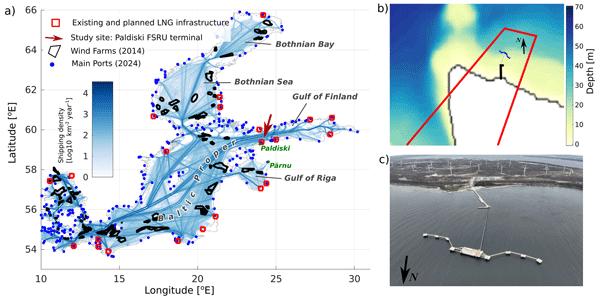
Beyond site-specific engineering concerns, the regional context of this study underscores the importance of robust metocean data. Across Europe, recent geopolitical shifts have prompted urgent efforts to diversify natural gas supply and bolster energy security – since early 2022, the EU has fast-tracked on the order of 30 new liquefied natural gas (LNG) import terminal projects (Ostrowski, 2022; Rymut and Mihaylov, 2025). In the Baltic region, countries are rapidly developing LNG infrastructure (including FSRU-based terminals) to reduce reliance on single pipeline routes and ensure reliable energy supply (Slakaityte et al., 2022). Estonia's planned LNG terminal near Paldiski, on the coast of the Gulf of Finland (Fig. 1), is such a case: the project was fast-tracked in 2022 as part of a broader strategy to improve the Baltic's energy resilience. Reliable metocean information is needed to assess structural safety and define permissible operating conditions. This high strategic importance places additional emphasis on getting the environmental design criteria right from the outset.
The Baltic Sea – and the Gulf of Finland in particular – presents unique metocean challenges that must be factored into design. This shallow, semi-enclosed sea has an irregular, fragmented coastline and complex bathymetry that produce highly localized wind, wave, and current patterns often harder to predict than those in the open ocean (Alenius et al., 1998; Soomere, 2005; Westerlund et al., 2019; Pellikka et al., 2023). The Gulf of Finland is a long, narrow sub-basin with complex coastal geometry. Its geometry and wind forcing can produce substantial non-tidal water-level variability, including storm-driven setup and the seiches (Medvedev and Kulikov, 2021; Barzandeh et al., 2025; Lorenz et al., 2025). The gulf's geometry limits the development of long-period swells; storms instead generate short-period, steep wind seas that – while lower in height than ocean swells – (Björkqvist et al., 2017; Kanarik et al., 2021; Björkqvist et al., 2021) can induce vigorous motions and cyclic loads on a moored FSRU. In winter, parts of the Gulf freeze over with seasonal sea ice, which dampens waves but introduces ice loading and operational constraints (Lu et al., 2024). These combined factors – non-tidal water level extremes, steep short waves, complex coastal currents, and periodic ice cover – create a demanding environment where high-resolution, site-specific metocean data and modeling are required to capture the full range of conditions for design and operations.
To meet these challenges, the present study leverages state-of-the-art long-term datasets and numerical modeling tools to characterize the metocean climate of the Paldiski site (Fig. 1). The Pakrineeme/Paldiski study site lies on the Pakri Peninsula, on Estonia's southern Gulf of Finland coast (Fig. 1), in a predominantly bedrock-controlled coastal setting. The FSRU berth has a representative water depth of approximately 16 m. Compared with the open Baltic Proper, the site is relatively sheltered from waves but remains susceptible to sea-level extremes and episodic wind-driven events. Modern metocean analyses increasingly rely on multi-decadal hindcasts and reanalyses to provide continuous, high-quality records of environmental parameters (Penalba et al., 2022; D'Agostini et al., 2024). Here we utilize roughly 30 years of data (spanning from the early 1990s to the 2020s) from open-access sources such as the Copernicus Marine Environment Monitoring Service (CMEMS) and ECMWF ERA5 Reanalysis, which offers specialized hindcast/reanalysis products for European regional seas. These include modeled time series of Baltic Sea wind speeds, wave heights, sea level variations, and currents that have been consistently processed and quality-controlled. Drawing on such extensive datasets ensures that both typical conditions and rare extremes are accounted for, providing a robust statistical basis for estimating the design environmental criteria.
In addition to analyzing historical data, we apply high-resolution numerical models to downscale and resolve local metocean conditions at the terminal site. A nested modeling approach is adopted: the regional Baltic wave model WAM (The Wamdi Group, 1988) provides boundary conditions to a fine-resolution nearshore wave model SWAN (Simulating WAves Nearshore; Booij et al., 1999) configured with detailed coastal bathymetry, thereby simulating how offshore waves transform as they propagate into the shallow gulf and around complex shoreline features. For hydrodynamics, we employ the NEMO (Nucleus for European Modelling of the Ocean; Madec et al., 2017) framework, NEMO-EST05 in particular, and the GETM (General Estuarine Transport Model; Burchard and Bolding, 2002) to reproduce local current patterns and sea level responses under various wind and pressure scenarios. NEMO-EST05 and GETM are independent downscaling simulations that both use boundary conditions from the CMEMS reanalysis. All these models have been calibrated for Baltic Sea conditions – accounting for factors like bottom friction and seasonal ice coverage – and their performance tested in past Baltic applications (Björkqvist et al., 2018; Kärnä et al., 2021; Raudsepp and Maljutenko, 2022; Björkqvist et al., 2024). By combining broad-scale reanalysis data with targeted local modeling, our study captures both large-scale climatic influences and fine-scale site effects in the metocean conditions.
To quantify the design extremes, we perform statistical extreme value analysis on the assembled data. Both block-maxima and peaks-over-threshold techniques are employed, fitting Generalized Extreme Value (GEV) distributions and Generalized Pareto Distributions (GPD) respectively to the long-term time series. This yields estimated return levels for various return periods (e.g. 10-year, 50-year, 100-year events) for each key parameter: wind speed, significant wave height, extreme high and low sea levels, and surface current speed. For the 50-year return period, for instance, our analysis indicates roughly a 23 m s−1 extreme wind, a 4.1 m significant wave height, a +1.5 m storm surge high water (and −0.7 m extreme low water), and about a 0.37 m s−1 surface current. The results provide marginal metocean return levels and uncertainty estimates that can be used as environmental input parameters for later design-load calculations.
A crucial aspect of our approach is the integration and distribution-based evaluation of multiple data sources, aligning with best practices in modern metocean studies. We compare model outputs and hindcast data against available observations – including satellite measurements (for example, altimeter-derived sea levels and scatterometer winds) and in situ records from local buoys and tide gauges – to assess consistency with the available observations. This multi-source comparison helps to quantify uncertainties and biases in the datasets, allowing us to correct the model predictions where necessary and improve confidence in the results. By fusing information from global reanalyses, regional models, remote sensing, and on-site measurements, the study minimizes the risk of relying on any single source. This data-driven, ensemble approach provides a multi-source characterization and identifies differences among the available estimates that can be trusted for engineering design and risk assessment in a high-stakes project.
The study addresses two linked questions. First, how can long-term observational, satellite, reanalysis, and high-resolution model datasets be combined to characterize metocean extremes at a specific coastal infrastructure site? Second, how do the resulting site-specific estimates relate to the spatial variability of extreme conditions across the Baltic Sea? We address these questions through a detailed assessment of the Pakrineeme/Paldiski FSRU site followed by a Baltic Sea-wide analysis of 50-year return levels. The purpose is not to introduce a new extreme-value method, but to demonstrate a transferable workflow in which regional datasets are evaluated and, where justified, locally adjusted for site-specific assessment, while spatially consistent regional products are used to provide the broader basin-scale context. The Baltic-wide results are therefore intended for regional comparison and screening; site-specific applications elsewhere require local observations, representativeness assessment, and, where necessary, local bias treatment.
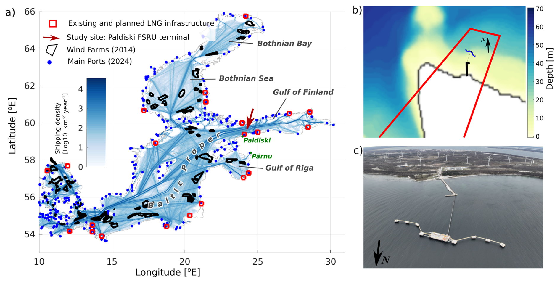
Figure 1Map of the Baltic Sea showing locations of various human activities (a). Existing and planned LNG infrastructure is redrawn from Gas Infrastructure Europe (2019), Global Energy Monitor (2024); offshore wind farms from European Marine Observation and Data Network (EMODnet; 2024a); main ports from EMODnet (2024b); and vessel traffic density from EMODnet (2024c). Panels (b) and (c) highlight LNG terminals and the location of the FSRU mooring quay. Panel (c) presents a drone photograph taken after construction. © Pärt (2026) Distributed under the Creative Commons Attribution 4.0 License. The red rectangle in panel (b) indicates the drone's field of view and the extent of the photograph shown in panel (c). GIE (2019) LNG infrastructure data reproduced under the Gas Infrastructure Europe usage terms (https://www.gie.eu, last access: 15 July 2025). GEM (2024) LNG infrastructure data courtesy of the Global Energy Monitor (https://globalenergymonitor.org, last access: 15 July 2025). EMODnet (2024a, b, c) offshore wind farms, ports, and vessel traffic density data provided by the European Marine Observation and Data Network (https://emodnet.ec.europa.eu, last access: 15 July 2025).
To support the metocean design basis for the proposed FSRU terminal near Paldiski, we employed a multi-source, multi-model approach combining observational datasets, global and regional reanalyses, and high-resolution numerical modeling. This section outlines the sources of environmental data and the methods used to derive local wind, sea level, wave, and current statistics, with particular focus on extreme value analysis. Where independent observations were available, model and reanalysis products were evaluated through comparisons with satellite and in situ measurements. This multi-source approach supports evaluation of dataset consistency and selection for the site-specific extreme-value assessment. For the site-specific assessment, data harmonization included aligning sea-level datasets to a common vertical datum, matching temporal resolution where direct model comparisons were required, and applying the observation-based wind and wave adjustments described below and in the Supplement. For the Baltic-wide assessment, the original gridded datasets were retained to preserve spatial consistency. The dataset-specific preprocessing is summarized in Table A1.
2.1 Wind Data and Modeling
Surface wind conditions were assessed using a combination of in situ measurements, satellite observations, and reanalysis products. Long-term wind observations from the Paldiski meteorological station (59.39° N, 24.04° E) were used as a reference (product ref. no. 13). This record spans from 1993 to 2021, with 3-hourly resolution until 2003 and hourly resolution thereafter.
ERA5 reanalysis (Hersbach et al., 2020; product ref. no. 3), with 10 m wind data at 0.25° resolution, served as the primary dataset for wind climatology and was used to drive wave and hydrodynamic models. Alternative regional reanalyses – COSMO-REA6 (Bollmeyer et al., 2015), BaltAn65+ (Luhamaa et al., 2011), and NORA3 (Solbrekke et al., 2021) – were evaluated but ultimately excluded due to systematic biases and inconsistencies when compared with coastal wind observations. COSMO-REA6 and BaltAn65+ consistently overestimated wind speeds during high wind events, with COSMO-REA6 also exhibiting unrealistic wind spikes. NORA3, despite its higher resolution, substantially underestimated high wind speeds. In contrast, ERA5 showed better agreement with in situ measurements throughout the year, justifying its selection as the primary wind dataset. Remote sensing data included ASCAT Level-3 scatterometer wind fields (MetOp A/B/C; 12.5 km resolution, 2007–present) (product ref. no. 4) and Sentinel-1 SAR Level-2 surface wind vectors (1 km resolution, 2017–present) (product ref. no. 5). Satellite wind data were extracted from open-sea locations approximately 15–20 km from the terminal site.
Using ASCAT wind speed measurements and ERA5 wind speed values a corrective function based on sigmoid was developed and applied for ERA5 wind speeds to reflect better measured open sea values in the region (Supplement, S1 Wind correction).
2.2 Sea Level Data and Modeling
Tide gauge measurements from the Paldiski North Port (59.34972° N, 24.0475° E) (product ref. no. 6) were used to evaluate sea level variability. Visual readings were available for 1993–2009, and hourly automated records for 2016–2021. Data gaps between 2010 and 2016 were filled using the CMEMS Baltic Sea Physics Reanalysis sea surface height time series (product ref. no. 1) at the nearest grid cell, after aligning the model series to the gauge datum and mean level over the overlapping period.
Satellite-derived sea surface height data included Level-3 along-track altimetry and gridded Level-4 products from multiple altimeter missions (Jason, Sentinel-3A, CryoSat-2, ENVISAT, etc.), obtained from the CMEMS database (product ref. no. 8 and 7).
Three model sources provided high-resolution sea level time series: (1) CMEMS Baltic Sea Physical Reanalysis (1 nmi resolution, 1993–2017) (product ref. no. 1), based on the NEMO-Nordic model; and two independent model simulations dynamically downscaled from the CMEMS reanalysis onto 0.5 nmi grids: (2) NEMO-EST05 hindcast (product ref. no. 9); (3) GETM barotropic surge model (Maljutenko and Raudsepp, 2019; product ref. no. 10). All sea level heights were converted to the same vertical datum as the Paldiski gauge (normalized to its 1993–2009 mean water level of +0.21 m) so that model and observed datasets could be consistently compared.
2.3 Wave Data and Modeling
Wave statistics were derived from two primary hindcast sources: (1) CMEMS Wave Reanalysis (WAM Cycle 4.6.2; 1 nmi grid, 1993–2020) (product ref. no. 2); (2) SWAN-EST05 high-resolution model (0.5 nmi grid, 2000–2009) (product ref. no. 12). The CMEMS hindcast was calibrated using short-term wave buoy observations (LainePoiss buoy (Alari et al., 2022), May–June 2022) collected near the terminal site (59.399° N, 24.103° E) (product ref. no. 11). A comparison of the CMEMS hindcast (product ref. no. 2) to the short-term in situ measurements (product ref. no. 11) revealed that the model had a slight high bias in wave heights. The summer 2022 buoy data, although limited, indicated that CMEMS over-predicted significant wave height by roughly 15 % during the comparison period. For the local analysis, significant wave heights were therefore reduced by 15 % and wave periods by 5 % using multiplicative scaling based on the near-site comparison (Supplement, Sect. S2 Wave correction). Because this adjustment is proportional to the original value, its absolute magnitude increases with wave height or period and it should not be interpreted as removal of a constant additive mean bias. Satellite altimeter data (Level-3, 2002–2020) (product ref. no. 14) were also used to assess significant wave height distributions.
2.4 Current Data and Modeling
Surface current were obtained from the CMEMS Baltic Sea Reanalysis (product ref. no. 1), available as daily means, and from the NEMO-EST05 high-resolution hindcast (product ref. no. 9), available at 1 h temporal resolution. For the distribution-based comparison in Fig. 2, the hourly NEMO-EST05 currents were averaged to daily means to match the temporal resolution of the CMEMS product. This averaging was used only for the direct comparison between the two datasets; the site-specific extreme-value analysis was based on the native hourly NEMO-EST05 current series.
2.5 Extreme value analysis framework
2.5.1 Site-specific Extreme Value Analysis (EVA)
To characterize metocean extremes, we applied statistical extreme value theory to the long-term time series. Two complementary methods were used: (1) Block Maxima Method, fitting Generalized Extreme Value (GEV) distributions to annual maxima (yearly values); (2) Peaks Over Threshold (POT), fitting Generalized Pareto Distributions (GPD) to exceedances over a high threshold. The main strengths of the Block Maxima Method are straightforward implementation and the absence of a threshold-selection requirement, making it convenient for consistent comparisons across variables and locations. However, retaining only one value per year discards other potentially informative storm events, while including maxima from relatively calm years. By retaining several independent extreme events per year, POT can use the available record more efficiently and potentially improve the precision of return-level estimates. Its main limitations are sensitivity to threshold selection and the need to separate dependent observations associated with the same storm (Jonathan and Ewans, 2013; Caruso and Marani, 2022). For the POT data a censoring time of 24 h was used to reduce dependence between exceedances associated with the same event . Model fits were performed via Maximum Likelihood Estimation (MLE). Special cases, including the Gumbel (GEV with shape = 0) and Exponential (GPD with shape = 0) distributions, were used where justified by the data. In practice, the GEV distribution provides additional flexibility by estimating the shape parameter from the annual maxima, allowing different tail behaviours to be represented. However, for records spanning only a few decades, the shape parameter may itself be weakly constrained and sensitive to individual extreme years. Consequently, the GEV was not assumed a priori to be superior to the simpler Gumbel distribution; the fitted distributions were evaluated together with their physical plausibility, and long-return-period estimates were interpreted cautiously (Jonathan and Ewans, 2013; Jonathan et al., 2021).
The return levels for 10, 20, 50, and 100-year periods were estimated for wind speed (product ref. no. 3, 13), significant wave height (product ref. no. 2, 12), sea level extremes (both high and low) (product ref. no. 1, 6, 9), and surface current speed (product ref. no. 9) at the LNG site (Fig. 1). A 100-year return level is a fitted probability statement, not an observed event that requires a 100-year record by definition. Nevertheless, estimating return levels beyond the length of the available record involves extrapolation of the fitted tail, and the associated uncertainty increases when only a few decades of extremes are available (Jonathan and Ewans, 2013; Jonathan et al., 2021). Therefore, we mainly focus on the 50-year estimates for local-regional comparison, and retain 100-year estimates only as explicitly qualified longer-return-period extrapolations. Selection of the final model and dataset for each parameter was based on best fit, physical plausibility, and consistency across data sources. The complete time series used for the site-specific assessment, together with the associated analysis scripts, are available in the data repository of Raudsepp et al. (2026b). Given the length and temporal resolution of these records, the manuscript presents their statistical distributions and extreme-value diagnostics rather than compressed plots of the complete time series.
2.5.2 Regional extreme value analysis
The regional extension of the EVA was designed to place the local FSRU site results within a broader Baltic Sea context while recognizing the different roles of the two analyses. At Paldiski, local observations and high-resolution modelling are used to evaluate the representativeness of the long-term datasets and support site-specific preprocessing. For the Baltic-wide analysis, the original gridded long-term datasets are retained so that a spatially consistent methodology can be applied across the basin. The correction factors derived at Paldiski are therefore not transferred to other locations, because their magnitude is expected to depend on local exposure, bathymetry, coastal geometry, and observation-to-grid representativeness While the EVA methods used here are standard, their consistent application across basin-wide, long-term metocean datasets allows the spatial distribution of return levels and associated uncertainty to be compared among different coastal and offshore infrastructure regions. This distinction is important because metocean extremes in the Baltic Sea are strongly controlled by basin geometry, fetch limitation, bathymetry, and sub-basin-scale circulation, and therefore local design values cannot be reliably generalized from one site to another. The regional estimates support preliminary comparison of rare-event exposure, while the local analysis addresses site-specific representativeness and preprocessing. However, return-level maps alone do not quantify the frequency or duration of calm conditions, operational weather windows or optimal siting. Those questions require additional time-series, directional, persistence and engineering analyses.
To extend the EVA regionally, we leverage comprehensive long-term datasets from the Copernicus Marine Service. The hindcast data underpinning our analysis include the Baltic Sea Multi-Year Physics Reanalysis for sea levels and currents (product ref. no. 1), and the Baltic Sea wave hindcast/reanalysis for wave heights (product ref. no. 2). These products provide a 31-year (1993–2024) homogeneous time series with daily temporal resolution (sea level and currents) and hourly (bulk wave parameters) at spatial resolution of 1 nautical mile, which are crucial for stable extreme statistics. Accordingly, the Baltic-wide current EVA is based on daily-mean surface currents and should be interpreted as a regional screening estimate rather than an estimate of sub-daily peak currents. Wind forcing is taken from the ERA5 global atmospheric reanalysis (hourly, ∼ 31 km grid) (product ref. no. 3), whose 10 m wind speeds have been rigorously validated and widely used for wave modeling in European seas (Hersbach et al., 2020). Recent evaluations indicate that using ERA5 winds can improve the representation of Baltic wave extremes, even if some regional reanalyses better capture the mean wave climate (Giudici et al., 2023).
The Baltic-wide EVA was performed using the original gridded long-term datasets in order to preserve spatial consistency. Block Maxima Method, fitting Generalized Extreme Value (GEV) distributions to annual maxima was used for the EVA. Annual-maxima GEV fitting provides a uniform framework for regional comparison. It avoids the location- and variable-specific threshold selection and storm-declustering diagnostics required by POT, simplifying regional implementation. This is a practical methodological choice – not evidence that POT is unsuitable – with the trade-off that additional extreme events within each year are discarded. To estimate the uncertainties in EVA of wind speed, wave height, sea level, and currents – a bootstrap resampling method was used. It is a non-parametric approach that involves resampling the original dataset (with replacement) many times and refitting the extreme value model each time. The method provides empirical distributions of return levels, from which confidence intervals can be derived. This is particularly useful when the sample size is small or when the distribution is skewed. We used this method to estimate the ranges of return values. We used 180 iterations, with the 2.5th and 97.5th percentiles as the lower and upper bounds of the results. Thus, the 95 % between them gives a full “confidence” interval.
The resulting maps should be interpreted as regional-scale estimates of metocean exposure rather than as locally bias-corrected design values. For site-specific applications elsewhere in the Baltic Sea, especially in nearshore or morphodynamically active areas, local validation against observations and local bias correction are required.
3.1 Wind Speed
A comparison of reanalysis and observed wind data (wind gusts excluded) indicated that the ERA5 10 m wind speeds (product ref. no. 3) underestimated the highest winds recorded at the Pakri coastal weather station (product ref. no. 13). After applying the correction function (see Supplement, Sect. S1 Wind correction), the distribution of ERA5 winds closely resembled open-sea conditions and aligned well with satellite scatterometer (ASCAT) measurements (product ref. no. 4) over the overlapping period 2012–2021, while still matching the high-end values recorded at Pakri (Fig. 2a, b). The Pakri station data, as expected for a land-based site, show a higher frequency of low wind speeds due to sheltering when winds blow from land, but they also captured a few extreme gusts that the coarser ASCAT sampling likely missed. Overall, the adjusted ERA5 dataset provides a representative wind climate for the offshore terminal location, capturing both the predominance of moderate maritime winds and the magnitude of rare storm peaks (Fig. 2a, b).
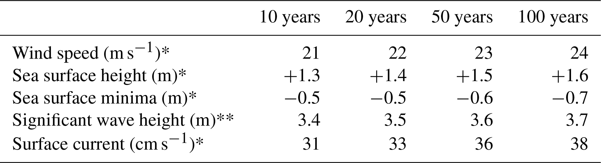
The fitted models describe the wind extremes well, including the highest recorded storm winds (Fig. 3a, b). The resulting 100-year return period wind speed – meaning the wind speed with a 1 % annual probability of exceedance – is approximately 24 m s−1 at 10 m elevation. Lower return period estimates follow accordingly (e.g. about 23 m s−1 for a 50-year return period; see Table 2). This ∼ 24 m s−1 extreme wind represents a critical design value for the FSRU terminal, defining the upper limit of wind loading that the mooring system and vessel must withstand.
3.2 Sea Level
Five different sea level datasets were evaluated to characterize water level variability at the site. These include the CMEMS Baltic Sea reanalysis (product ref. no. 1; 1 nmi resolution), the subregional NEMO-EST05 model (product ref. no. 9; 0.5 nmi resolution), the regional GETM model (product ref. no. 10; 0.5 nmi resolution), along with satellite altimetry (instantaneous along-track Level 3 and daily-averaged gridded Level 4 products) (product ref. no. 8 and 7), and the tide gauge observations at Paldiski (product ref. no. 6). Figure 2c, d illustrates the probability distributions of sea level from these sources over their common period. The three continuous hindcasts (CMEMS, NEMO-EST05, and GETM), which provide hourly sea level time series for 1993–2017, show very similar distributions and are broadly in agreement with the statistical behavior of the Paldiski gauge record (which spans 1993–2009 with gaps). In contrast, the satellite-based records are either smoothed or sparse: the Level 4 product, with its daily averaging, smooths out short-lived peaks and thus underrepresents extreme high or low water events, whereas the instantaneous Level 3 altimeter data capture the full range of variability but contain relatively few data points near the study area. These differences in sampling density are reflected in the lengths of the distribution curves in Fig. 2c, d. When examining the upper and lower tails of the sea level distributions on a logarithmic scale (Fig. 2d), we find generally good agreement, but with some differences in extreme values across datasets. In the high-water (positive) tail, the CMEMS hindcast (product ref. no. 1) tends to predict slightly more frequent very high water levels than the NEMO-EST05 (product ref. no. 9) and GETM (product ref. no. 10) models. For instance, near the observed maximum sea levels, the CMEMS curve extends a bit further, suggesting a higher likelihood of extreme surge events in that dataset. The GETM and NEMO hindcasts yield somewhat lower extreme probabilities, but all three model-based datasets exhibit a similarly steep drop-off in the tail (Fig. 2c, d), indicating they capture the rarity of extreme surges in the Gulf of Finland. In summary, while the lower-to-moderate sea level range is consistently represented across all sources, the CMEMS data provide a somewhat more conservative estimate of the highest water levels, making it a useful dataset for extreme analysis.
For extreme high sea levels, we focused on the model hindcasts and reanalysis for return period estimation, while using the Paldiski tide gauge data (product ref. no. 6) for context and validation. The annual maximum sea level in each year of the CMEMS (product ref. no. 1) and NEMO-EST05 (product ref. no. 9) series was extracted and fitted to GEV distributions. Both models yielded consistent results, with Gumbel-type fits adequately describing the upper tail (Fig. 3c–e). The CMEMS hindcast produced slightly higher estimates for a given return period, and we adopted those as a conservative choice for design criteria. Notably, the largest storm surge on record in these series corresponds to the January 2005 cyclone “Gudrun,” which produced a water level of roughly +1.5 m at the site (Suursaar and Sooäär, 2007). In the CMEMS data, this event falls around the 100-year return level on the fitted curve, whereas in the NEMO-EST05 data it appears closer to a 50-year event based on extrapolation. The extreme value analysis yields a 100-year return high water level of about +1.6 m relative to the local mean sea level (Fig. 3c). This value is taken as the extreme storm surge level for design purposes.
The annual minimum sea level from each year was used for the block-maxima analysis (since the lowest water level of each year represents the most extreme drop). This approach was chosen over a POT method because the very lowest value on record was a clear outlier that made threshold-based fitting unstable. The GEV fits to the annual minima from both the CMEMS (product ref. no. 1) and NEMO hindcasts (product ref. no. 9) suggest nearly identical low-water extremes. The estimated 100-year return period minimum sea level is approximately −0.8 m (i.e. 0.8 m below the mean sea level baseline). In practical terms, such an extreme low sea level, while infrequent, must be considered in FSRU design to ensure sufficient draught and flexible connections during extreme low-water events. The symmetry between the +1.6 m high and −0.8 m low centennial levels highlights the Gulf's propensity for greater positive storm surges than negative seiches (since the basin's geometry and prevailing winds favor high-water extremes (Medvedev and Kulikov, 2021).
3.3 Waves
To characterize the wave climate, we compared significant wave height data from multiple sources, emphasizing long-term model hindcasts as the basis for statistics. The primary datasets were the CMEMS Baltic Sea wave reanalysis (product ref. no. 2) and a high-resolution SWAN hindcast (product ref. no. 12). Available observations were limited to a short-term wave buoy deployment near the site in summer 2022 (product ref. no. 11) and a sparse set of satellite altimeter passes (Level-3 data, product ref. no. 8), which are insufficient to capture extreme wave conditions. As shown in Fig. 2e, f, the two models exhibit generally consistent wave-height distributions after the correction factor was applied to the CMEMS Baltic Sea wave reanalysis (Supplement, Sect. S2 Wave correction). Both suggest that most of the time the significant wave height is relatively modest (<2 m) consistent with the fetch-limited nature of the gulf. For significant wave heights above approximately 0.4 m, however, the SWAN-EST05 distribution is generally higher than that of the CMEMS wave reanalysis. Because the datasets differ in model configuration, spatial resolution, and forcing, the comparison does not allow this difference to be attributed to a single cause (Najafzadeh et al., 2021, 2024). Overall, both model datasets identify a similar wave-climate regime dominated by short-period wind seas, and provide complementary estimates for the extreme-wave analysis.
Despite the different spatial resolution and time span of the two wave models, their extreme value statistics turned out to be in strong agreement. GEV fits to the annual maxima from CMEMS (product ref. no. 2) and SWAN-EST05 (product ref. no. 12) provided a better fit than the Gumbel distribution. For the POT analysis, the GPD fits with an exponential tail, adequately captured the upper-end behaviour of both datasets (Figs. 3j, k; A1j, k). For example, the statistically estimated 100-year return significant wave height is on the order of 3.6 m based on these fits.
3.4 Currents
Observations of surface currents in the Gulf of Finland are sparse, so we relied on hydrodynamic model data to assess current speed statistics. Two model sources were considered: the NEMO-EST05 high-resolution Baltic Sea circulation hindcast (1993–2017) (product ref. no. 9) and the surface current product from the CMEMS reanalysis (daily outputs over a similar period) (product ref. no. 1). To enable a direct comparison, the NEMO-EST05 1 h data (nemoh) were averaged into daily means (nemod) to match the temporal resolution of CMEMS. The resulting distributions of surface current speed from the two models are plotted in Fig. 2g, h on a logarithmic scale. Both datasets indicate that currents at the proposed terminal location are generally weak. Typical surface flow speeds are on the order of a few centimeters per second, and even the upper quantiles remain modest (on the order of 0.25–0.35 m s−1). The two hindcasts agree well on this overall magnitude: their probability density curves overlap closely through most of the range. Both models paint a consistent picture of a low-energy surface circulation regime at the site, driven primarily by wind and seiche events in the semi-enclosed gulf. More generally, Baltic Sea surface circulation reflects the combined contributions of geostrophic and ageostrophic currents, with wind and sea-level variability contributing to the spatial circulation patterns (Barzandeh et al., 2024). Recent data-driven analyses of daily surface-current fields further indicate strong spatial heterogeneity, with wind providing important basin-scale predictive information while coastal, strait, and boundary regions exhibit stronger local constraints and day-to-day complexity (Barzandeh et al., 2026a, b).
For the site-specific extreme-current analysis, annual maximum surface current speeds were extracted from the the native 1 h NEMO-EST05 hindcast (considering the top 1 m layer average) (product ref. no. 9) rather than from the daily-averaged series used for the inter-model comparison in Fig. 2. The NEMO-based extreme value curves suggest that 100-year return period surface currents are on the order of 0.4 m s−1. The GEV fit for the annual maxima had a positive shape parameter (indicating an upward-curving tail in Fig. 3k), while the exponential-tail POT fit captured the few highest current events well (Fig. A1k); both methods yielded similar 100-year estimates around 0.39–0.43 m s−1. It should be noted that these values come with larger uncertainty bands compared to the other parameters, mainly due to the lack of long-term current measurements for validation and the inherent variability in modeling coastal currents. We interpret ∼ 0.4 m s−1 as a reasonable upper-bound estimate for the site's surface current under present climate conditions. Although this extreme current speed is relatively low in comparison to open-ocean currents, in combination with high winds and waves it could still contribute to the total environmental force on the moored FSRU.
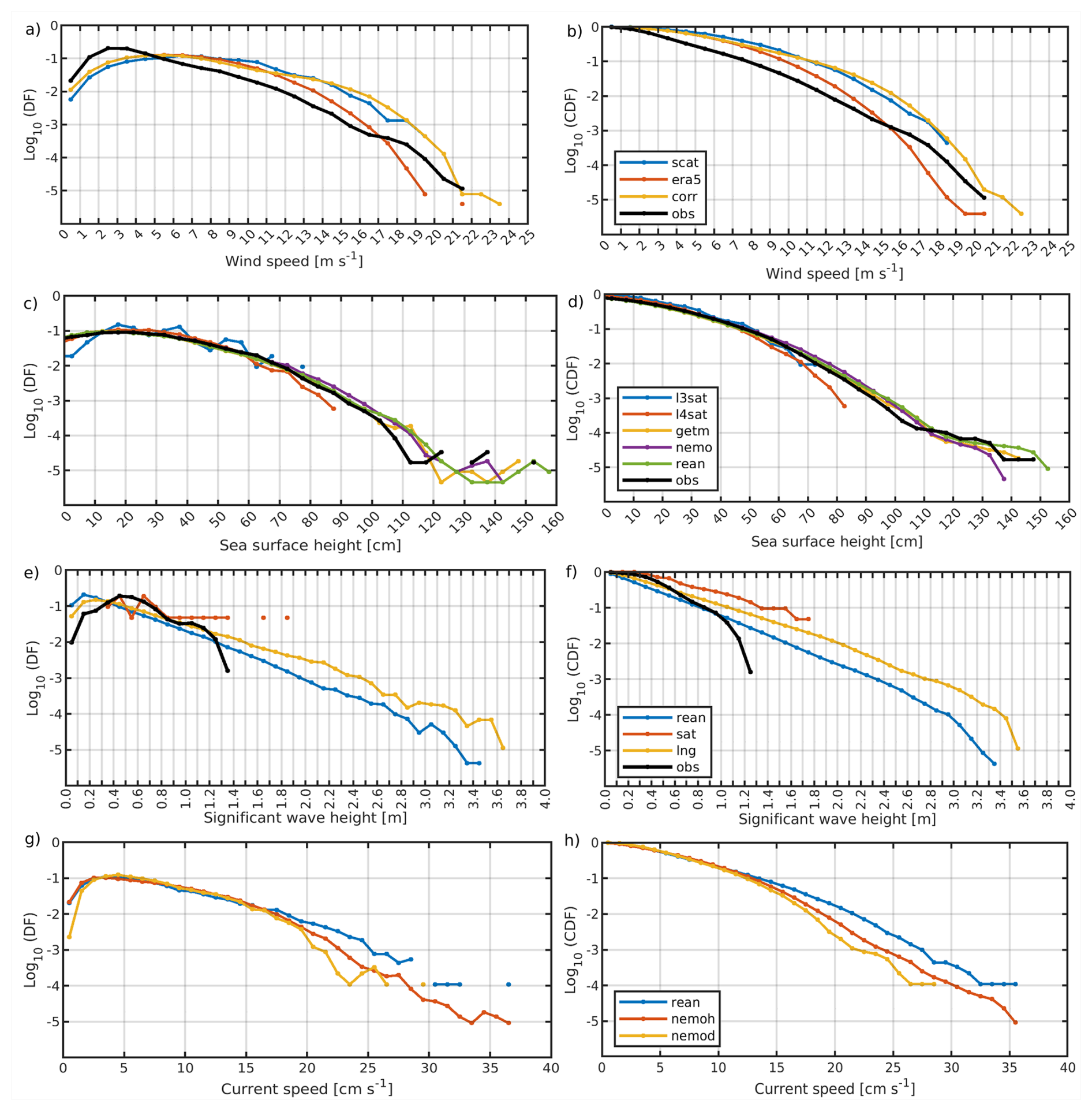
Figure 2Log scale density distribution functions (DF) (left column) and cumulative distribution function (CDF) (right column) of wind speed (a, b; product ref. nos. 3, 4, 13; product 3 is also shown after the site-specific wind adjustment), sea surface height (c, d; product ref. nos. 1, 6, 7, 8, 9, 10), and significant wave height (e, f; product ref. nos. 2, 14, 12, 11) sea surface current speed (g, h; product ref. nos. 1, 9) of various data sources at the terminal location. Temporal coverage differs among the data sources and is reported in Sect. 2.1–2.4 and in Table A1.
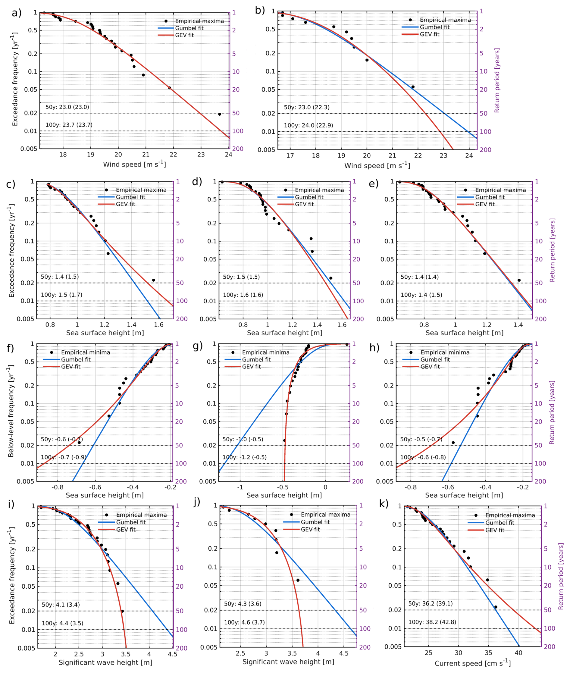
Figure 3Generalized Extreme Value (GEV) and Gumbel distributions fitted to annual maxima and minima of key oceanographic variables: wind speed (a–b) (product ref. no. 3 – a, 13 – b), sea surface height maxima (c–e) (product ref. no. 1 – c, 6 – d, 9 – e), sea surface height minima (f–h) (product ref. no. 1 – f, 6 – g, 9 – h), significant wave height maxima (panels i–j) (product ref. no. 2 – i, 12 – j), and surface current speed maxima (k) (product ref. no. 9 – k). Horizontal dashed lines denote the 50- and 100-year return periods, with corresponding return levels for Gumbel fits shown (GEV estimates indicated in brackets).
Table 2An overview of the return levels for the environmental variables for return periods of 10, 20, 50 and 100 years at LNG site. One asterisk corresponds to Gumbel and two asterisks to GEV fit.
3.5 Extension of the Extreme value analysis to the whole Baltic Sea
Having used the Paldiski case to assess how regional products represent local extremes relative to observations and higher-resolution datasets, we extend the same EVA framework across the Baltic Sea to examine the spatial variability of 50-year return levels and their uncertainties (Fig. 4).
The wind speed values are higher over the sea area than over the land (Fig. 4a). This is because of the absence of orographic restrictions over the sea area. Over the sea, extreme wind speeds show a north-south and coastal-offshore variability. In the south-western Baltic Sea, the ERA5-based 50-year return level reaches approximately 28 m s−1. The corresponding 95 % confidence interval is wide, with an uncertainty range of up to about 10 m s−1 in some grid cells, indicating substantial uncertainty in the fitted tail distribution. The most severe Baltic windstorms, often following a track across the open sea, have produced 10 min mean wind speeds above 30 m s−1 over water (Björkqvist et al., 2020). For example, the January 2019 storm's peak winds reached 32.5 m s−1 over the Baltic Proper, driving the extreme waves (Björkqvist et al., 2020).
Our analysis shows high extreme values of the wave height and wave period over the eastern Baltic Proper (Fig. 4c–f). The 50-year significant-wave-height return level reaches approximately 10 m in the most exposed parts of the Baltic Proper. The 95 % confidence-interval width locally exceeds 5 m, so these values should be interpreted as regional screening estimates rather than site-specific design values. A significant wave height of 8.1 m was measured in the northern Baltic – the highest on record – with hindcasts suggesting waves up to 9 m in the Bothnian Sea (Björkqvist et al., 2020).
The Baltic-wide wind-speed return levels are based on ERA5 10 m hourly wind fields. They therefore represent gridded hourly 10 m wind-speed return levels, not gusts, 10 min station wind maxima, or wind speeds adjusted to turbine-hub height or vessel-superstructure height. This distinction is important because temporal averaging, vertical level, and spatial resolution all affect the magnitude of estimated extremes. The mapped values may therefore appear low when compared with observed gusts or short-duration storm maxima.
The large confidence intervals in parts of the south-western Baltic Sea are caused mainly by the limited number of years that are covered by the data set, strong interannual variability, and sensitivity of the unconstrained GEV shape parameter. The uncertainty is therefore partly statistical and partly structural. In addition, ERA5 is known to smooth small-scale wind maxima and may underestimate high-wind events in the Baltic Sea. Consequently, the ERA5-based wind map should be interpreted as an internally consistent regional screening product. Local design applications require validation against local observations and, where appropriate, local bias correction.
Sea surface current speeds are high at the coastal sea, where locally, the extreme values could reach 1 m s−1 (Fig. 4g). Simultaneously, the uncertainties of these extreme values are almost 2 m s−1 (Fig. 4h).
Storm surge (sea level) extremes display particularly strong spatial variability due to the Baltic's complex geometry and bathymetry. We should note that long-term mean sea level was not removed from the analysed data. Extreme sea levels in the Baltic Sea are driven by wind-driven surge, atmospheric pressure, and seiche oscillations. The highest surges occur when strong winds align with the basin's long axis and push water into narrow bays or gulfs. Maximum sea level anomalies are expected in the eastern Gulf of Finland and the Gulf of Riga (Fig. 4i). There, the extreme sea level corresponding to the 50-year return period could be as high as 1.3 m. At the end of the Gulf of Finland, uncertainties of the extreme value estimate are also high, reaching up to 1.3 m (Fig. 4j). In the Gulf of Riga the uncertainties remain below 0.8 m (Fig. 4j). In the Gulf of Riga, the town of Pärnu has suffered two record surges: 2.53 m in 1967 and 2.75 m in January 2005 (Lorenz et al., 2025; Suursaar and Sooäär, 2007) – the latter being one of the highest reliably measured sea levels in the entire Baltic during the last century.
The uncertainties in the maximum sea-level anomaly map should be interpreted with caution. The Baltic wide sea level EVA is based on daily gridded CMEMS physical reanalysis output, whereas local tide gauges and site-specific studies may use hourly or higher-frequency records. Daily fields can smooth short-lived storm-surge peaks and may underestimate the highest instantaneous water levels. In narrow sub-basins such as the eastern Gulf of Finland and the Gulf of Riga, annual maxima are also strongly influenced by a small number of major storm-surge events, which makes the fitted GEV tail sensitive to individual years. The confidence intervals shown in the map therefore represent statistical uncertainty of the gridded daily-field EVA, but not the full uncertainty associated with temporal resolution, vertical datum, local bathymetry, or gauge-to-grid representativeness.
Correspondingly, minimum sea levels were found to be around −0.7 m for a 50-year return period at the site of the LNG terminal (Table 2). The Baltic Sea wide estimates provide minimum sea levels down to −0.4 m (Fig. 4k) with maximum uncertainty of up to 0.3 m (Fig. 4l) corresponding to a return period of 50-years. The discrepancy could be related to the fact that hourly sea level values were used at the LNG while daily values for the whole Baltic Sea. We note that uncertainty in these return level estimates is considerable, owing to the relatively short observational records (30 years) and natural variability. We like to note that extreme values of high sea level are significantly higher than low sea levels relative to zero sea level.
Metocean criteria derived from local and Baltic-wide EVA provide environmental inputs for subsequent, separate engineering analyses for the engineering specifications for mooring systems, platform freeboards, breakwater heights, and operational limits. For example, the calculated extreme significant wave height guides the required height of mooring dolphins and fenders to avoid collision or overtopping in a storm. The extreme wind speed and currents inform the loads on the FSRU's mooring lines and the tension capacity needed to keep it in place during a gale. Even extreme low water levels (e.g. −0.7 m in our 50-year estimate) are important, as they determine the minimum under-keel clearance and the design of intake/outlet systems for the FSRU.
3.6 Synthesis of site-specific and Baltic Sea-wide assessments
Comparison of the site-specific and Baltic Sea-wide results demonstrates the importance of local exposure and temporal resolution when translating regional extreme-value estimates to infrastructure applications. At the Paldiski FSRU site, the 50-year return levels are approximately 23 m s−1 for wind speed, 4.1 m for significant wave height, 0.37 m s−1 for surface current speed, and +1.5 m and −0.7 m for maximum and minimum sea level, respectively. The regional assessment shows considerably larger wind, wave, and current extremes in more exposed parts of the Baltic Sea, with wind-speed return levels reaching approximately 28 m s−1, significant wave heights approaching 10 m in the Baltic Proper, and surface currents locally approaching 1 m s−1. This confirms that the Paldiski site is relatively sheltered with respect to waves and currents compared with the most exposed Baltic regions.
Sea level shows a different spatial behaviour. The largest positive regional anomalies occur in geometrically constrained sub-basins such as the Gulf of Finland and Gulf of Riga. The site-specific sea-level extremes are also larger than those obtained from the Baltic-wide daily fields at the corresponding regional scale, particularly for low water. This difference is partly attributable to temporal resolution, because the site-specific analysis uses hourly data whereas the regional assessment uses daily fields that can smooth short-lived extrema. The comparison therefore demonstrates that the Baltic-wide maps provide a consistent regional screening framework, whereas infrastructure design requires site-specific data and evaluation at an appropriate temporal and spatial resolution.
3.7 Model and data limitations
Beyond the statistical uncertainty of the fitted return levels shown in Fig. 4, the assessment is affected by limitations in model formulation and input data. We consider three main sources: the absence of two-way wave–circulation coupling, the use of fixed bathymetry without morphodynamic changes, and the choice and spatial resolution of atmospheric forcing.
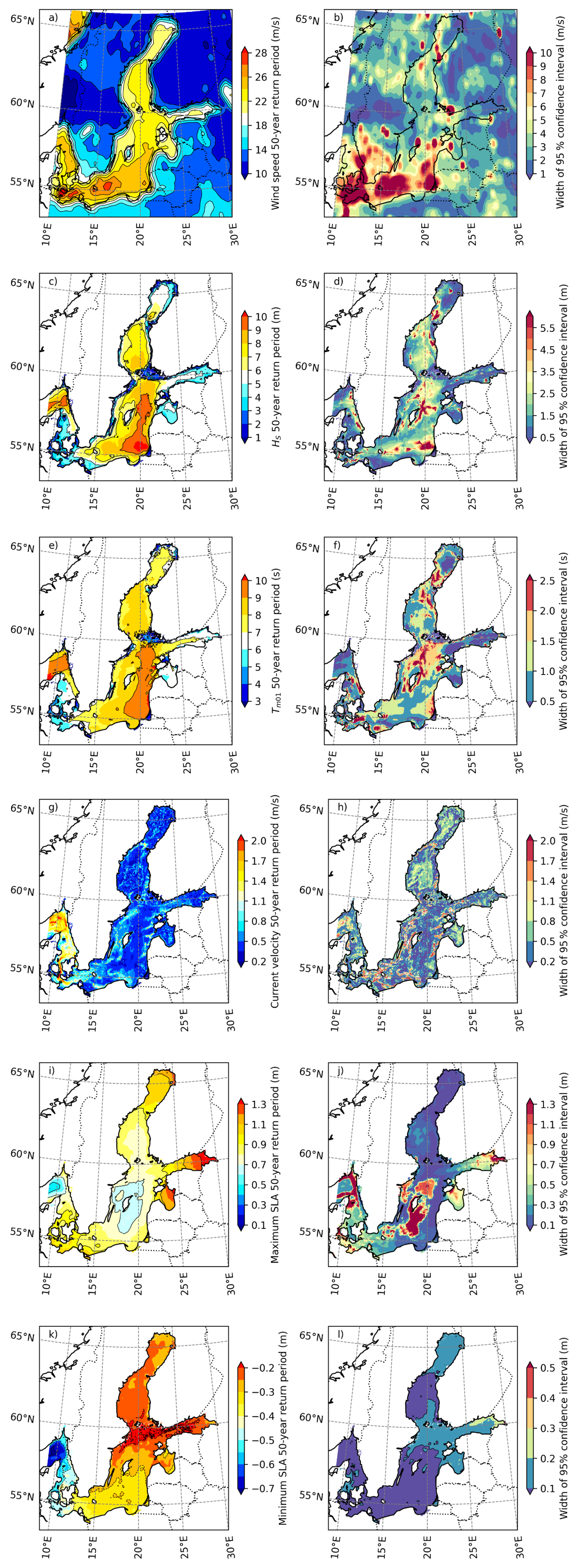
Figure 4Extreme values corresponding to the return period of 50-years (left panels) and the uncertainties of their estimates (right panels). Wind speed (a, b) from product ref. no. 3, significant wave height (c, d) and peak period (e, f) from product ref. no. 2, current velocity (g, h) from product ref. no. 1, and maximum (i, j) and minimum (k, l) sea level anomaly from product ref. no. 1.
The wave and hydrodynamic datasets used in this study are not fully two-way coupled. The CMEMS multi-year Baltic Sea wave product is based on WAM, while the corresponding physical reanalysis is based on NEMO; these long-term production systems are run independently without exchange of wave, current, or waterlevel parameters. Similarly, the high resolution SWAN-EST05 and NEMO-EST05 datasets were used here as separate wave and hydrodynamic products. This means that current-induced wave refraction, water-level-dependent wave transformation, wave-induced set-up, radiation stress effects, and Stokes drift feedback on currents are not fully represented in the long-term extreme value analysis. Explicit wave forcing can also modify ocean-side stress, Stokes–Coriolis forcing, turbulence, and upper-ocean mixing, demonstrating that the absence of wave feedbacks can affect the simulated hydrodynamic state (Haapaniemi et al., 2026).
The possible effect of this decoupling was assessed qualitatively and by scale analysis. At the FSRU site, currents are generally weak, and the estimated 50-year return surface current is approximately 0.37 m s−1. Previous Baltic Sea sensitivity experiments have shown that including modelled currents usually produces small changes in significant wave height, although local changes can become larger during strong-current events, especially in coastal areas and in the Gulf of Finland (Kanarik et al., 2021). The berth is also relatively deep compared with the estimated design wave height: using a representative berth depth of about 16 m and a 50-year significant wave height of 4.1 m gives , where h is local water depth, indicating that the local wave extreme is not expected to be primarily depth limited. Water-level variations therefore influence local wave transformation but are unlikely to dominate the significant wave height return level at the berth.
The uncertainty introduced by missing coupling is considered a structural model uncertainty. For significant wave height, we estimate that the effect is likely small for the marginal return levels, but individual storm events with strong opposing currents may produce deviations of order 0.1–0.3 m and, in rare local cases, up to approximately 0.5–0.6 m. This uncertainty is comparable in magnitude to the site-specific multiplicative wave-height adjustment and the spread between the independent wave datasets. Previous Baltic Sea sensitivity experiments with WAM forced by NEMO surface currents showed that current effects on the wave field are generally small: changes exceeding 0.10 m in significant wave height or 1 s in peak period occurred only in limited areas and typically less than 3 % of the time, although event-scale changes up to about 0.6 m in maximum significant wave height can occur locally, especially near coasts and in the Gulf of Finland (Kanarik et al., 2021). The decoupled approach is therefore considered adequate for estimating marginal long-term return levels, but fully coupled event based simulations are recommended for final engineering design and operational limit assessment.
The present study focuses on long-term metocean extremes derived from observational, reanalysis, and numerical model datasets. Sediment transport and morphological change were not explicitly simulated. The wave and hydrodynamic products used in the EVA are based on fixed bathymetry and therefore do not include feedbacks from erosion, deposition, nearshore bar migration, dredging, or seabed recovery after storms. This limitation is particularly relevant in very shallow sandy nearshore areas, where changes in seabed morphology can modify wave breaking, wave refraction, current patterns, under-keel clearance, and local water-level impacts.
For the Pakrineeme FSRU site, this source of uncertainty is considered limited for the marginal return levels reported here. The terminal is located at the Pakri Peninsula, a predominantly bedrock-controlled coastal setting associated with the North Estonian limestone klint. The berth is also situated at a relatively deep jetty rather than directly on a sandy surf-zone coast. Existing project documentation indicates that the jetty is mainly pile supported and that no breakwaters were planned, while local dredging was carried out to secure the required berthing depth. These local seabed modifications are relevant for construction, maintenance dredging, and detailed engineering design, but they are not expected to dominate the long-term wind, wave, current, and sea level return levels estimated in this study.
For the Baltic-wide assessment, the uncertainty is larger. The regional EVA maps are based on gridded metocean products and should not be interpreted as resolving site-specific morphodynamics in the first nearshore grid cells. Along sandy and morphodynamically active coasts, especially in the southern and south-eastern Baltic Sea, erosion, deposition, nearshore bar migration, and harbour-related sediment interruption can substantially alter local bathymetry and therefore local metocean conditions. Baltic Sea coastal change studies show that erosion and accretion depend strongly on hydrodynamic conditions, wave climate, wave approach angle, sediment availability, and sediment compartments; sedimentary shores can be sensitive to relatively small variations in these drivers (Weisse et al., 2021). In the south-eastern Baltic, studies of the Curonian Spit show active nearshore sandbar switching and beach foredune response on storm, interannual, and decadal timescales, demonstrating that sandy nearshore morphology can change substantially over periods relevant to infrastructure planning (Janušaitė et al., 2023). The confidence intervals shown in the Baltic-wide maps (Fig. 4) represent statistical uncertainty of the extreme-value estimates, but they do not include morphological uncertainty. Consequently, the Baltic-wide results should be used as regional screening information, while detailed design at sandy nearshore sites requires local bathymetric surveys and sediment-transport or morphodynamic modelling.
The Baltic-wide results show that metocean design conditions are not spatially uniform and that the dominant hazard type differs between sub-basins (Fig. 4). Exposed areas of the Baltic Proper are characterized by the largest wave-height and wave-period extremes, whereas the highest positive sea-level anomalies occur in geometrically constrained regions such as the eastern Gulf of Finland and the Gulf of Riga. In contrast, the Paldiski FSRU site is relatively sheltered with respect to wave exposure compared with the Baltic Proper, but remains sensitive to sea level extremes and episodic wind driven events. This contrast demonstrates why a single regional design criterion is insufficient for Baltic Sea infrastructure planning. The uncertainty maps further show that some areas with high return levels also have broad confidence intervals, indicating where additional observations or higher-resolution modelling would most improve future risk assessments.
The Baltic-wide EVA results should be interpreted as regional-scale return levels of the uncorrected datasets. The confidence intervals shown in Fig. 4 describe statistical uncertainty from the EVA procedure, but they do not include uncertainty associated with spatially varying model bias. At the Paldiski site, the observation-based adjustments applied to the local analysis were approximately 5 %–10 % for wind speed, 15 % for significant wave height, and 5 % for wave period. These values are provided only as an example of the magnitude of model − observation differences at one coastal location. They were not applied to the Baltic-wide analysis and should not be interpreted as basin-wide uncertainty estimates, because the magnitude and potentially the sign of model bias may vary with local exposure, bathymetry, coastal geometry, and observation-to-grid representativeness. Site-specific applications therefore require evaluation and, where justified, local adjustment.
The choice of atmospheric forcing is an additional source of structural uncertainty in the Baltic-wide EVA. Although CERRA (Ridal et al., 2024) provides a substantially higher horizontal resolution than ERA5, it was not used in the present analysis because the marine products used here are ERA5-forced. A CERRA based wind map alone would not reduce uncertainty in the coupled interpretation of metocean extremes unless the corresponding wave and hydrodynamic fields were also generated using the same atmospheric forcing. This is particularly important because the CMEMS Baltic wave hindcast has been tuned for ERA5 wind forcing. Therefore, the Baltic-wide maps presented here should be interpreted as internally consistent ERA5-forced regional screening products.
Future work should assess the sensitivity of Baltic Sea metocean extremes to atmospheric forcing by comparing ERA5, CERRA, and possibly other regional reanalysis forced wave and hydrodynamic hindcasts. Such a study would require basin-wide validation against wind stations, satellite winds, wave buoys, tide gauges, and current observations. The present study does not perform this full forcing sensitivity experiment, and the resulting uncertainty is now explicitly acknowledged.
Finally, the broader strategic relevance of extreme value studies in the Baltic Sea must be underscored. The Baltic region is characterized by sensitive environmental conditions and heavily used sea routes (Fig. 1a) (for commerce and increasingly for energy transport). Geopolitical factors – such as shifting trade patterns, military considerations, and transnational energy projects – mean that infrastructure robustness is part of national resilience. For example, the disruption of one LNG terminal by an extreme storm could have ripple effects on multiple countries' energy supply. Therefore, the Baltic-wide EVA provides a regional screening framework for comparing the relative exposure of existing and prospective infrastructure areas to metocean extremes. It is not intended to identify operational refuge locations, towing destinations, or optimal terminal sites, which would require additional analyses of persistence, directionality, accessibility, navigation constraints, and engineering requirements.
This study provides an integrated assessment of metocean extremes for the planned FSRU terminal on the Estonian coast of the Gulf of Finland and places the local results in a Baltic Sea-wide context. The statistical methods used are established EVA approaches; the scientific contribution lies in the harmonized integration of multiple long-term observational, satellite, reanalysis, and high-resolution model datasets, together with distribution-based evaluation against available observations and independent model products, to derive consistent extreme-value estimates for wind, sea level, waves, and currents. For the FSRU site, the resulting 50-year return levels are approximately 23 m s−1 for wind speed, +1.5 and −0.7 m for sea-surface-height maxima and minima, 4.1 m for significant wave height, and 0.37 m s−1 for surface current speed. These values provide a site-specific metocean characterization for a sheltered but strategically important coastal location.
Extending the analysis to the entire Baltic Sea reveals strong spatial contrasts in 50-year return levels and their uncertainties. The largest wave extremes occur in exposed parts of the Baltic Proper, whereas the largest positive sea-level anomalies occur in constrained sub-basins such as the Gulf of Finland and the Gulf of Riga. These results show that metocean risk cannot be inferred from a single location or parameter, but requires a spatially resolved, multi-variable assessment. The basin-wide uncertainty estimates further identify areas where present datasets are less robust and where additional observations or higher-resolution modelling would be most valuable. The study therefore contributes not by proposing a new EVA method, but by providing a transparent, transferable framework for linking evaluated multi-source metocean datasets, local infrastructure needs, and regional-scale hazard assessment in the Baltic Sea. The Baltic-wide maps should therefore be used as regional screening products, while detailed design at other Baltic Sea sites requires local validation and site-specific bias assessment.
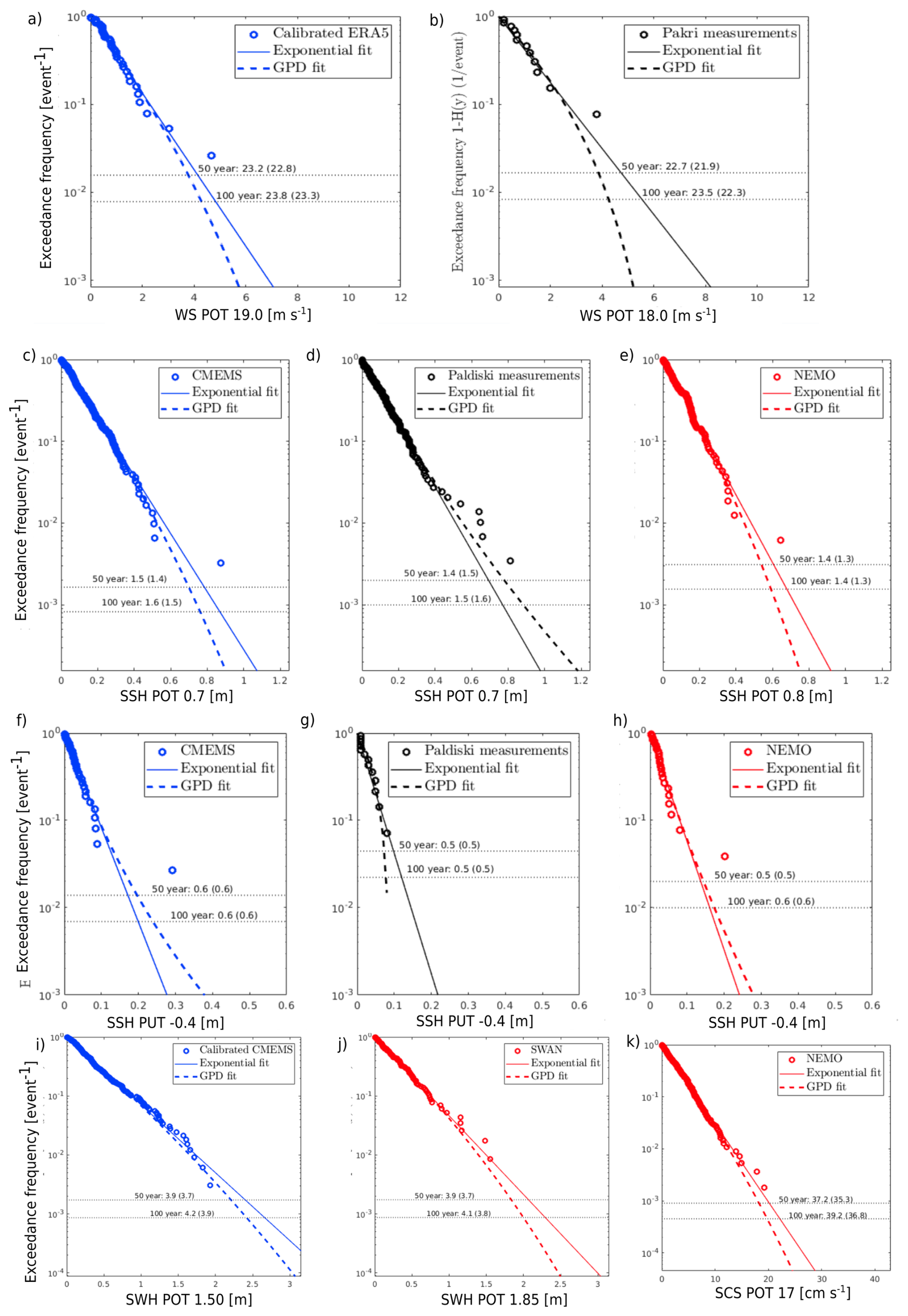
Figure A1Generalized Pareto Distribution (GPD) and Exponential distribution fits to peaks over/under thresholds (POT/PUT) for selected oceanographic variables: wind speed (WS ymax, panels a–b) (product ref. no. 3 – a, 13 – b), sea surface height maxima (SSH ymax, panels c–e) (product ref. no. 1 – c, 6 – d, 9 – e), sea surface height minima (SSH ymin, panels f–h) (product ref. no. 1 – f, 6 – g, 9 – h), significant wave height maxima (SWH ymax, panels i–j) (product ref. no. 2 – i, 12 – j), and surface current speed maxima (SCS ymax, panel k) (product ref. no. 9 – k). For SSH minima, positive values represent depressions below the threshold (i.e., negative sea level excursions). Horizontal lines indicate the 50- and 100-year return periods, with corresponding return levels shown (GPD estimates indicated in brackets).
Table A1Datasets used in the study, their temporal and spatial resolution, and study-specific pre-processing.
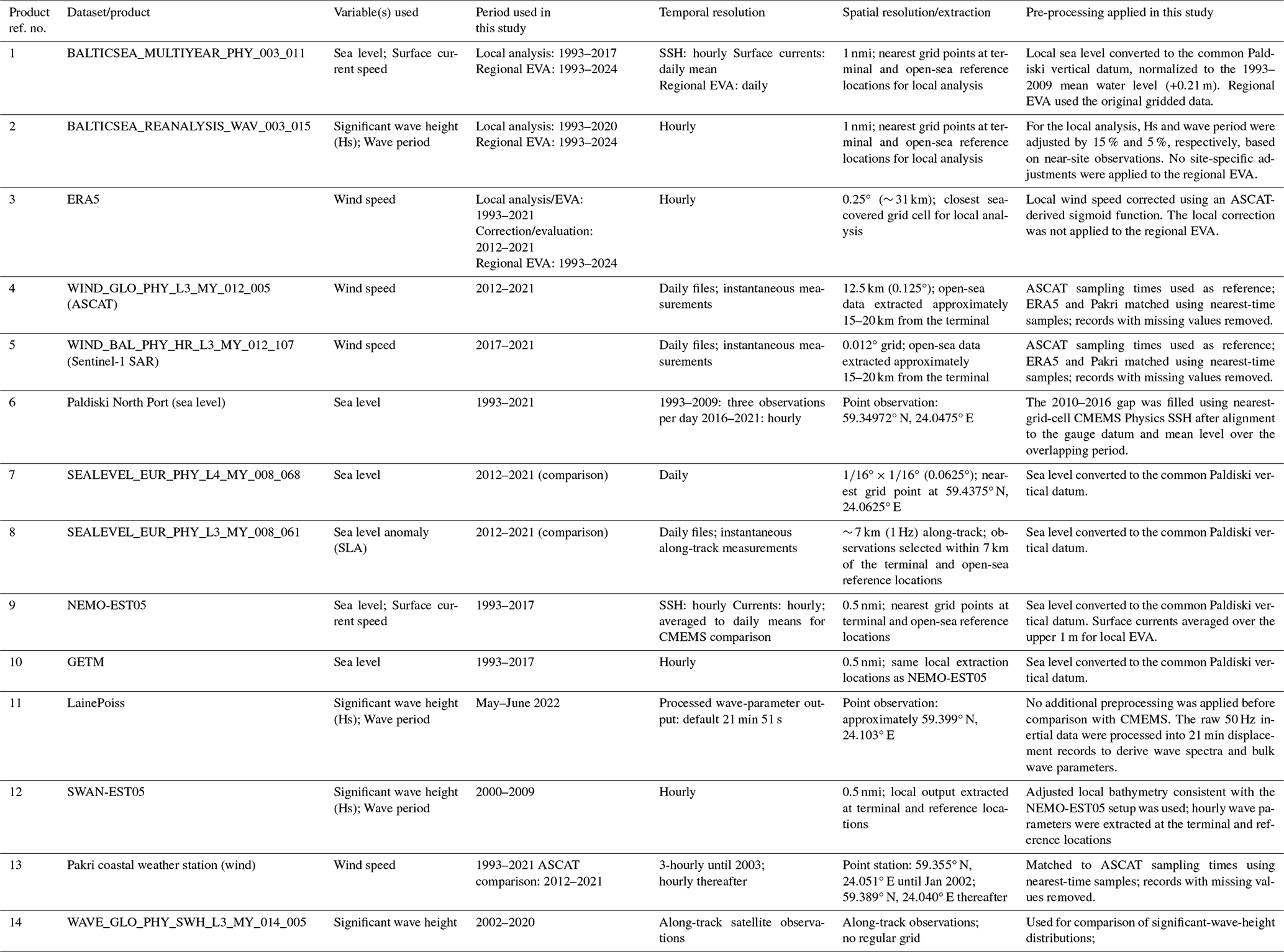
This study is based on public databases and the references are listed in Table 1. The datasets and software codebases are published in Zenodo data repositories (https://doi.org/10.5281/zenodo.20378599, Raudsepp et al., 2026a and https://doi.org/10.5281/zenodo.20356006, Raudsepp et al., 2026b).
The supplement related to this article is available online at https://doi.org/10.5194/sp-7-osr10-14-2026-supplement.
UR led the research, drafted the original manuscript, and contributed to manuscript review and editing. IM, JVB, AB, SR, AM, and SP curated the data and conducted the analysis. SP and KV conducted the wave observations. PL, VA, and RU contributed to the conceptualization and design of the study. All authors participated in scientific discussions and reviewed the manuscript.
The contact author has declared that neither of the authors has any competing interests.
The Copernicus Marine Service offering is regularly updated to ensure it remains at the forefront of user requirements. In this process, some products may undergo replacement or renaming, leading to the removal of certain product IDs from the catalogue. If readers have any questions or require assistance regarding these modifications, please feel free to reach out to the Copernicus Marine Service user support team for further guidance. They will be able to provide the necessary information to address concerns and find suitable alternatives.
Publisher's note: Copernicus Publications remains neutral with regard to jurisdictional claims made in the text, published maps, institutional affiliations, or any other geographical representation in this paper. The authors bear the ultimate responsibility for providing appropriate place names. Views expressed in the text are those of the authors and do not necessarily reflect the views of the publisher.
OpenAI's GPT-4o model was used to assist with initial drafting sections of the manuscript. All content was reviewed, verified, and approved by the authors.
This paper was edited by Joanna Staneva and reviewed by three anonymous referees.
Alari, V., Björkqvist, J.-V., Kaldvee, V., Mölder, K., Rikka, S., Kask-Korb, A., Vahter, K., Pärt, S., Vidjajev, N., and Tõnisson, H.: LainePoiss® – A Lightweight and Ice-Resistant Wave Buoy, J. Atmos. Ocean. Tech., 39, 573–594, https://doi.org/10.1175/JTECH-D-21-0091.1, 2022.
Alenius, P., Myrberg, K., and Nekrasov, A.: The physical oceanography of the Gulf of Finland: a review, Boreal Environ. Res, 3, 97–125, 1998.
Allen, T. R., McLeod, G., and Hutt, S.: Sea level rise exposure assessment of US East Coast cargo container terminals, Marit. Policy Manag., 49, 577–599, https://doi.org/10.1080/03088839.2021.1903597, 2022.
Bailey, B. H. and Freedman, J. M.: Developments in metocean information in support of US offshore wind energy and the ocean sciences, Oceanography, 37, 30–41, https://doi.org/10.5670/oceanog.2024.503, 2024.
Ballarotta, M., Pujol, M.-I., and SL-TAC team: EU Copernicus Marine Service Quality Information Document for European Seas Gridded L4 Sea Surface Heights and Derived Variables Reprocessed (1993–ongoing), SEALEVEL_EUR_PHY_L4_MY_008_068, Issue 13.0, Mercator Ocean International, https://documentation.marine.copernicus.eu/QUID/CMEMS-SL-QUID-008-032-068.pdf (last access: 15 July 2025), 2025a.
Ballarotta, M., Pujol, M.-I., and SL-TAC team: EU Copernicus Marine Service Quality Information Document for European Seas Along Track L 3 Sea Surface Heights Reprocessed 1993 Ongoing Tailored For Data Assimilation, SEALEVEL_EUR_PHY_L3_MY_008_061, Issue 13.0, Mercator Ocean International, https://documentation.marine.copernicus.eu/QUID/CMEMS-SL-QUID-008-032-068.pdf (last access: 15 July 2025), 2025b
Barzandeh, A., Maljutenko, I., Rikka, S., Lagemaa, P., Männik, A., Uiboupin, R., and Raudsepp, U.: Sea surface circulation in the Baltic Sea: decomposed components and pattern recognition, Scientific Reports, 14, 18649, https://doi.org/10.1038/s41598-024-69463-8, 2024.
Barzandeh, A., Maljutenko, I., Rikka, S., and Raudsepp, U.: sciCUN: A deep learning model for daily sea surface current fields inference – A case study of the Gulf of Riga, Ocean Model., 201, 102693, https://doi.org/10.1016/j.ocemod.2026.102693, 2026a.
Barzandeh, A., Manss, C., Stahl, F., Maljutenko, I., Rikka, S., and Raudsepp, U.: Data-Driven Emulation of Numerically Simulated Baltic Sea Surface Currents With a Deep Convolutional U-Net: Explainability and Potential Forecast Skill, J. Geophys. Res. Mach. Learn. Comput., 3, e2026JH001321, https://doi.org/10.1029/2026JH001321, 2026b.
Barzandeh, A., Ličer, M., Rus, M., Kristan, M., Maljutenko, I., Elken, J., Lagemaa, P., and Uiboupin, R.: Application of the HIDRA2 deep-learning model for sea level forecasting along the Estonian coast of the Baltic Sea, Ocean Sci., 21, 1315–1327, https://doi.org/10.5194/os-21-1315-2025, 2025.
Bitner-Gregersen, E. M.: Joint met-ocean description for design and operations of marine structures, Appl. Ocean Res., 51, 279–292, https://doi.org/10.1016/j.apor.2015.01.007, 2015.
Björkqvist, J.-V., Tuomi, L., Fortelius, C., Pettersson, H., Tikka, K., and Kahma, K. K.: Improved estimates of nearshore wave conditions in the Gulf of Finland, J. Mar. Syst., 171, 43–53, https://doi.org/10.1016/j.jmarsys.2016.07.005, 2017.
Björkqvist, J.-V., Lukas, I., Alari, V., van Vledder, G. Ph., Hulst, S., Pettersson, H., Behrens, A., and Männik, A.: Comparing a 41-year model hindcast with decades of wave measurements from the Baltic Sea, Ocean Eng., 152, 57-71, https://doi.org/10.1016/j.oceaneng.2018.01.048, 2018.
Björkqvist, J.-V., Rikka, S., Alari, V., Männik, A., Tuomi, L., and Pettersson, H.: Wave height return periods from combined measurement–model data: a Baltic Sea case study, Nat. Hazards Earth Syst. Sci., 20, 3593–3609, https://doi.org/10.5194/nhess-20-3593-2020, 2020.
Björkqvist, J.-V., Pärt, S., Alari, V., Rikka, S., Lindgren, E., and Tuomi, L.: Swell hindcast statistics for the Baltic Sea, Ocean Sci., 17, 1815–1829, https://doi.org/10.5194/os-17-1815-2021, 2021.
Björkqvist, J.-V., Kanarik, H., Tuomi, L., Niskanen, L., and Kankainen, M.: Event-based wave statistics for the Baltic Sea, in: 8th edition of the Copernicus Ocean State Report (OSR8), edited by: von Schuckmann, K., Moreira, L., Grégoire, M., Marcos, M., Staneva, J., Brasseur, P., Garric, G., Lionello, P., Karstensen, J., and Neukermans, G., Copernicus Publications, State Planet, 4-osr8, 10, https://doi.org/10.5194/sp-4-osr8-10-2024, 2024.
Bollmeyer, C., Keller, J. D., Ohlwein, C., Wahl, S., Crewell, S., Friederichs, P., Hense, A., Keune, J., Kneifel, S., Pscheidt, I., Redl, S., and Steinke, S.: Towards a high-resolution regional reanalysis for the European CORDEX domain, Q. J. Roy. Meteor. Soc., 141, 1–15, https://doi.org/10.1002/qj.2486, 2015.
Booij, N., Ris, R. C., and Holthuijsen, L. H.: A third-generation wave model for coastal regions: 1. Model description and validation, J. Geophys. Res.-Oceans, 104, 7649–7666; https://doi.org/10.1029/98JC02622, 1999.
Burchard, H. and Bolding, K. K.: GETM, a General Estuarine Transport Model, Technical Report, European Commission, Joint Research Centre, Institute for Environment and Sustainability, https://publications.jrc.ec.europa.eu/repository/handle/JRC23237 (last access: 22 September 2026), 2002.
Caruso, M. F. and Marani, M.: Extreme-coastal-water-level estimation and projection: a comparison of statistical methods, Nat. Hazards Earth Syst. Sci., 22, 1109–1128, https://doi.org/10.5194/nhess-22-1109-2022, 2022.
Charles, E. and Ollivier, A.: EU Copernicus Marine Service Quality Information Document for the Global Ocean L3 Significant Wave Height From Reprocessed Satellite Measurements, WAVE_GLO_PHY_SWH_L3_MY_014_005, Issue 2.0, Mercator Ocean International, https://documentation.marine.copernicus.eu/QUID/CMEMS-WAVE-QUID-014-005.pdf (last access: 15 September 2026), 2026.
Cheynet, E., Li, L., and Jiang, Z.: Metocean conditions at two Norwegian sites for development of offshore wind farms, Renew. Energy, 224, 120184, https://doi.org/10.1016/j.renene.2024.120184, 2024.
CLS, IFREMER, OCEANSCOPE, De Carlo, M., Piollé, J.-F., and Husson, R.: EU Copernicus Marine Service Product User Manual for the High-resolution L3 Sea Surface Wind from MY Satellite Measurements over the Baltic Sea, WIND_BAL_PHY_HR_L3_MY_012_107, Issue 1.2, Mercator Ocean International, https://documentation.marine.copernicus.eu/PUM/CMEMS-WIND-PUM-012-100to109.pdf (last access: 15 July 2025), 2025.
Copernicus Climate Change Service: Complete ERA5 global atmospheric reanalysis, Copernicus Climate Change Service (C3S) Climate Data Store (CDS) [data set], https://doi.org/10.24381/cds.143582cf, 2023.
D'Agostini, A., Campos, R. M., and Soares, C. G.: Assessments of multiple metocean forecasts in the North Atlantic Ocean, Ocean Eng., 312, 119199, https://doi.org/10.1016/j.oceaneng.2024.119199, 2024.
Driesenaar, T., de Kloe, J., Belmonte Rivas, M., Giesen, R., Stoffelen, A., Bentamy, A., Hackett, B., and Garcia Hermosa, I.: EU Copernicus Marine Service Quality Information Document for Global Ocean Daily Gridded Reprocessed L3 Sea Surface Winds from Scatterometer, WIND_GLO_PHY_L3_MY_012_005, Issue 1.19, Mercator Ocean International, https://documentation.marine.copernicus.eu/QUID/CMEMS-WIND-QUID-012-002-005.pdf (last access: 15 July 2025), 2024a.
Driesenaar, T., de Kloe, J., Belmonte Rivas, M., Stoffelen, A., Forneris, V., van Zadelhoff, G.-J., and Giesen, R.: EU Copernicus Marine Service Product User Manual for the Global Ocean Daily Gridded Reprocessed L3 Sea Surface Winds from Scatterometer, WIND_GLO_PHY_L3_MY_012_005, Issue 2.26, Mercator Ocean International, https://documentation.marine.copernicus.eu/PUM/CMEMS-WIND-PUM-012-002-005.pdf (last access: 15 July 2025), 2024b.
EMODnet: Centro Tecnológico del Mar – Fundación CETMAR: EMODnet Human Activities – Energy – Offshore Wind Farms, EMODNET_HA_ENERGY_WINDFARMS, Version 2024, European Marine Observation and Data Network, https://emodnet.ec.europa.eu/geonetwork/srv/eng/catalog.search#/metadata/8201070b-4b0b-4d54-8910-abcea5dce57f (last access: 15 July 2025), 2024a.
EMODnet: Eurofish International Organisation and Cogea Srl: EMODnet Human Activities – Main Ports, Goods-Passengers-Vessels Traffic (annual aggregation, 1997–2024), EMODNET_HA_MainPorts_Traffic_20241112, Version 2024, European Marine Observation and Data Network, https://emodnet.ec.europa.eu/geonetwork/srv/eng/catalog.search#/metadata/379d0425-8924-4a41-a088-1a002d2ea748 (last access: 15 July 2025), 2024b.
EMODnet: Falco, L. and Adnams, W.: EMODnet Human Activities – Vessel Density Map (EU waters, 2017–2023), EMODNET_HA_Vessel_Density_Map_20240304, Version 2024, European Marine Observation and Data Network, https://emodnet.ec.europa.eu/geonetwork/srv/eng/catalog.search#/metadata/0f2f3ff1-30ef-49e1-96e7-8ca78d58a07c (last access: 15 July 2025), 2024c.
EU Copernicus Marine Service Product: Baltic Sea Wave Hindcast, Marine Data Store (MDS) [data set], https://doi.org/10.48670/moi-00014, 2024a.
EU Copernicus Marine Service Product: Global Ocean Daily Gridded Reprocessed L3 Sea Surface Winds from Scatterometer, Marine Data Store (MDS) [data set], https://doi.org/10.48670/moi-00183, 2024b.
EU Copernicus Marine Service Product: Baltic Sea Physics Reanalysis, Marine Data Store (MDS) [data set], https://doi.org/10.48670/moi-00013, 2025a.
EU Copernicus Marine Service Product: High-resolution L3 Sea Surface Wind from MY Satellite Measurements over the Baltic Sea, Marine Data Store (MDS) [data set], https://doi.org/10.48670/mds-00340, 2025b.
EU Copernicus Marine Service Product: European Seas Gridded L 4 Sea Surface Heights And Derived Variables Reprocessed 1993 Ongoing, Marine Data Store (MDS) [data set], https://doi.org/10.48670/moi-00141, 2025c.
EU Copernicus Marine Service Product: European Seas Along Track L3 Sea Surface Heights Reprocessed 1993 Ongoing Tailored For Data Assimilation, Marine Data Store (MDS) [data set], https://doi.org/10.48670/moi-00139, 2025d.
EU Copernicus Marine Service Product: Global Ocean L3 Significant Wave Height from Reprocessed Satellite Measurements, Marine Data Store (MDS) [data set], https://doi.org/10.48670/moi-00176, 2025e.
Global Energy Monitor (GEM): Global Gas Infrastructure Tracker – Pipelines (Release: December 2024) and LNG Terminals (Release: September 2024), https://globalenergymonitor.org/projects/global-gas-infrastructure-tracker (last access: 15 July 2025), 2024.
Gas Infrastructure Europe (GIE): GIE LNG Map 2019 existing, under construction, planned, and proposed LNG terminals across Europe, Version: May 2019, https://www.gie.eu/download/maps/2019/GIE_LNG_2019_A0_1189x841_FULL_Final3.pdf (last access: 15 July 2025), 2019.
Giudici, A., Jankowski, M. Z., Männikus, R., Najafzadeh, F., Suursaar, Ü., and Soomere, T.: A comparison of Baltic Sea wave properties simulated using two modelled wind data sets, Estuar. Coast. Shelf Sci., 290, 108401, https://doi.org/10.1016/j.ecss.2023.108401, 2023
Haapaniemi, V., Tuomi, L., Björkqvist, J.-V., Twelves, A., Murawski, J., Kanarik, H., Falahat, S., Westerlund, A., and Nummelin, A.: Surface wave impacts on turbulent roughness length parameterization, Ocean Model., 202, 102742, https://doi.org/10.1016/j.ocemod.2026.102742, 2026.
Hersbach, H., Bell, B., Berrisford, P., Hirahara, S., Horányi, A., Muñoz‐Sabater, J., Nicolas, J., Peubey, C., Radu, R., Schepers, D., Simmons, A., Soci, C., Abdalla, S., Abellan, X., Balsamo, G., Bechtold, P., Biavati, G., Bidlot, J., Bonavita, M., De Chiara, G., Dahlgren, P., Dee, D., Diamantakis, M., Dragani, R., Flemming, J., Forbes, R., Fuentes, M., Geer, A., Haimberger, L., Healy, S., Hogan, R.J., Hólm, E., Janisková, M., Keeley, S., Laloyaux, P., Lopez, P., Lupu, C., Radnoti, G., de Rosnay, P., Rozum, I., Vamborg, F., Villaume S., and Thépaut, J.-N.: The ERA5 global reanalysis, Q. J. Roy. Meteor. Soc., 146, 1999–2049, https://doi.org/10.1002/qj.3803, 2020.
Ho, R.-T.: Engineering Considerations for Offshore FSRU LNG Receiving Terminals, in: Offshore Technology Conference, Houston, Texas, USA, May 2008, https://doi.org/10.4043/19439-MS, 2008.
Husson, R., De Carlo, M., Colin, A., Peureux, C., Singhoff, H., Nedellec, M., Mouche, A., Piolle, J.-F., and Cevaer, T.: EU Copernicus Marine Service Quality Information Document for High-resolution L3 Sea Surface Wind from MY Satellite Measurements over the Baltic Sea, WIND_BAL_PHY_HR_L3_MY_012_107, Issue 1.2, Mercator Ocean International, https://documentation.marine.copernicus.eu/QUID/CMEMS-WIND-QUID-012-100to109.pdf (last access: 15 July 2025), 2025.
Janušaitė, R., Jarmalavičius, D., Pupienis, D., Žilinskas, G., and Jukna, L.: Nearshore sandbar switching episodes and their relationship with coastal erosion at the Curonian Spit, Baltic Sea, Oceanologia, 65, 71–85, https://doi.org/10.1016/j.oceano.2021.11.004, 2023.
Jonathan, P. and Ewans, K.: Statistical modelling of extreme ocean environments for marine design: A review, Ocean Eng., 62, 91–109, https://doi.org/10.1016/j.oceaneng.2013.01.004, 2013.
Jonathan, P., Randell, D., Wadsworth, J., and Tawn, J.: Uncertainties in return values from extreme value analysis of peaks over threshold using the generalised Pareto distribution, Ocean Eng., 220, 107725, https://doi.org/10.1016/j.oceaneng.2020.107725, 2021.
Kanarik, H., Tuomi, L., Björkqvist, J.-V., and Kärnä, T.: Improving Baltic Sea wave forecasts using modelled surface currents, Ocean Dynam., 71, 635–653, https://doi.org/10.1007/s10236-021-01455-y, 2021.
Kanarik, H., Tuomi, L., and Lindgren, E..: EU Copernicus Marine Service Quality Information Document for the Baltic Sea Wave Hindcast Product, BALTICSEA_REANALYSIS_WAV_003_015, Issue 2.0, Mercator Ocean International, https://documentation.marine.copernicus.eu/QUID/CMEMS-BAL-QUID-003-015.pdf (last access: 11 June 2025), 2024.
Kärnä, T., Ljungemyr, P., Falahat, S., Ringgaard, I., Axell, L., Korabel, V., Murawski, J., Maljutenko, I., Lindenthal, A., Jandt-Scheelke, S., Verjovkina, S., Lorkowski, I., Lagemaa, P., She, J., Tuomi, L., Nord, A., and Huess, V.: Nemo-Nordic 2.0: operational marine forecast model for the Baltic Sea, Geosci. Model Dev., 14, 5731–5749, https://doi.org/10.5194/gmd-14-5731-2021, 2021.
Keevallik, S. and Soomere, T.: Seasonal and diurnal variations of wind parameters at Pakri, Estonian J. Eng., 15, 227–239, https://doi.org/10.3176/eng.2009.3.06, 2009.
Lindgren, E., Tuomi, L., Kanarik, H., and Huess, V.: EU Copernicus Marine Service Product User for the Baltic Sea Wave Hindcast Product, BALTICSEA_REANALYSIS_WAV_003_015, Issue 2.0, Mercator Ocean International, https://documentation.marine.copernicus.eu/PUM/CMEMS-BAL-PUM-003-015.pdf (last access: 11 June 2025), 2024.
Lorenz, M., Viigand, K., and Gräwe, U.: Untangling the waves: decomposing extreme sea levels in a non-tidal basin, the Baltic Sea, Nat. Hazards Earth Syst. Sci., 25, 1439–1458, https://doi.org/10.5194/nhess-25-1439-2025, 2025.
Lu, L., Kondratenko, A., Kulkarni, K., Li, F., Kujala, P., and Musharraf, M.: An Investigation of Winter Navigation and Icebreaker Needs in the Ice-Infested Water: The Gulf of Finland and the Gulf of Riga, in: International Conference on Offshore Mechanics and Arctic Engineering, V006T07A006, https://doi.org/10.1115/OMAE2024-127955, 2024.
Luhamaa, A., Kimmel, K., Männik, A., and Rõõm, R.: High resolution re-analysis for the Baltic Sea region during 1965–2005 period, Clim. Dynam., 36, 727–738, https://doi.org/10.1007/s00382-010-0842-y, 2011.
Madec, G., Bourdallé-Badie, R., Bouttier, P.-A., Bricaud, C., Bruciaferri, D., Calvert, D., Chanut, J., Clementi, E., Coward, A., and Delrosso, D.: NEMO ocean engine, Zenodo, https://doi.org/10.5281/zenodo.3248739, 2017.
Maljutenko, I. and Raudsepp, U: Long-term mean, interannual and seasonal circulation in the Gulf of Finland – the wide salt wedge estuary or gulf type ROFI, J. Mar. Syst., 195, 1–19, https://doi.org/10.1016/j.jmarsys.2019.03.004, 2019.
Medvedev, I. P. and Kulikov, E. A.: Extreme Storm Surges in the Gulf of Finland: Frequency-Spectral Properties and the Influence of Low-Frequency Sea Level Oscillations, Oceanology, 61, 459–468, https://doi.org/10.1134/S0001437021040111, 2021.
Mrozowski, P.: Method for determining location of FSRU terminal, TransNav Int. J. Mar. Navig. Saf. Sea Transp., 18, https://doi.org/10.12716/1001.18.01.05, 2024.
Najafzadeh, F., Jankowski, M. Z., Giudici, A., Männikus, R., Suursaar, Ü., Viška, M., and Soomere, T.: Spatiotemporal variability of wave climate in the Gulf of Riga, Oceanologia, 66, 56–77, https://doi.org/10.1016/j.oceano.2023.11.001, 2024.
Najafzadeh, F., Kudryavtseva, N., and Soomere, T.: Effects of large-scale atmospheric circulation on the Baltic Sea wave climate: application of the EOF method on multi-mission satellite altimetry data, Clim. Dynam., 57, 3465–3478, https://doi.org/10.1007/s00382-021-05874-x, 2021.
Nigou, A. and Ollivier, A.: EU Copernicus Marine Service Product User Manual for the Global Ocean L3 Significant Wave Height From Reprocessed Satellite Measurements, WAVE_GLO_PHY_SWH_L3_MY_014_005, Issue 1.0, Mercator Ocean International, https://documentation.marine.copernicus.eu/PUM/CMEMS-WAVE-PUM-014-005.pdf (last access: 15 September 2026), 2026.
Ostrowski, W.: The twenty years' crisis of European energy security: Central and Eastern Europe and the US, Geopolitics, 27, 875–897, https://doi.org/10.1080/14650045.2020.1835863, 2022.
Panteleit, T., Verjovkina, S., Jandt-Scheelke, S., Spruch, L., and Huess, V.: EU Copernicus Marine Service Quality Information Document for the Baltic Sea Physics Reanalysis Product, BALTICSEA_MULTIYEAR_PHY_003_011, Issue 4.1, Mercator Ocean International, https://documentation.marine.copernicus.eu/QUID/CMEMS-BAL-QUID-003-011.pdf (last access: 11 June 2025), 2025.
Pärt, S., Björkqvist, J. V., Alari, V., Maljutenko, I., and Uiboupin, R.: An ocean–wave–trajectory forecasting system for the eastern Baltic Sea: Validation against drifting buoys and implementation for oil spill modeling, Mar. Pollut. Bull., 195, 115497, https://doi.org/10.1016/j.marpolbul.2023.115497, 2023.
Pellikka, H., Johansson, M. M., Nordman, M., and Ruosteenoja, K.: Probabilistic projections and past trends of sea level rise in Finland, Nat. Hazards Earth Syst. Sci., 23, 1613–1630, https://doi.org/10.5194/nhess-23-1613-2023, 2023.
Penalba, M., Aizpurua, J. I., Martinez-Perurena, A., and Iglesias, G.: A data-driven long-term metocean data forecasting approach for the design of marine renewable energy systems, Renew. Sustain. Energy Rev., 167, 112751, https://doi.org/10.1016/j.rser.2022.112751, 2022.
Pujol, M.-I.: EU Copernicus Marine Service Product User Manual for European Seas Gridded L4 Sea Surface Heights and Derived Variables Reprocessed (1993–ongoing), SEALEVEL_EUR_PHY_L4_MY_008_068, Issue 10.0, Mercator Ocean International, https://documentation.marine.copernicus.eu/PUM/CMEMS-SL-PUM-008-032-068.pdf (last access: 15 July 2025), 2025a.
Pujol, M.-I.: EU Copernicus Marine Service Product User Manual for European Seas Along-Track L3 Sea Surface Heights Reprocessed (1993–ongoing) Tailored For Data Assimilation, SEALEVEL_EUR_PHY_L3_MY_008_061, Issue 10.0, Mercator Ocean International, https://documentation.marine.copernicus.eu/PUM/CMEMS-SL-PUM-008-032-068.pdf (last access: 15 July 2025), 2025b
Raudsepp, U. and Maljutenko, I.: A method for assessment of the general circulation model quality using the K-means clustering algorithm: a case study with GETM v2.5, Geosci. Model Dev., 15, 535–551, https://doi.org/10.5194/gmd-15-535-2022, 2022.
Raudsepp, U., Maljutenko, I., Björkqvist, J.-V., Barzandeh, A., Rikka, S., Männik, A., Pärt, S., Alari, V., Vahter, K., and Uiboupin, R.: 50-Year return level datasets for the Baltic Sea, Version v1, Zenodo [data set], https://doi.org/10.5281/zenodo.20378599, 2026a
Raudsepp, U., Maljutenko, I., Björkqvist, J.-V., Barzandeh, A., Rikka, S., Männik, A., Pärt, S., Lagemaa, P., Alari, V., Vahter, K., and Uiboupin, R.: Metocean Data and Analysis Scripts for FSRU Terminal Planning on the Estonian Coast of the Gulf of Finland, Zenodo [data set], https://doi.org/10.5281/zenodo.20356006, 2026b
Ridal, M., Bazile, E., Le Moigne, P., Randriamampianina, R., Schimanke, S., Andrae, U., Berggren, L., Brousseau, P., Dahlgren, P., Edvinsson, L., El-Said, A., Glinton, M., Hagelin, S., Hopsch, S., Isaksson, L., Medeiros, P., Olsson, E., Unden, P., and Wang, Z. Q.: CERRA, the CopernicusEuropean Regional Reanalysis system, Q. J. Roy. Meteor. Soc., 150, 3385–3411, https://doi.org/10.1002/qj.4764, 2024.
Ringgaard, I., Korabel, V., Spruch, L., Lindenthal, A., and Huess, V.: EU Copernicus Marine Service Product User Manual for the Baltic Sea Physics Reanalysis Product, BALTICSEA_MULTIYEAR_PHY_003_011, Issue 1.0, Mercator Ocean International, https://documentation.marine.copernicus.eu/PUM/CMEMS-BAL-PUM-003-011-012.pdf (last access: 11 June 2025), 2024.
Robertson, B., Dunkle, G., Gadasi, J., Garcia-Medina, G., and Yang, Z.: Holistic marine energy resource assessments: A wave and offshore wind perspective of metocean conditions, Renew. Energy, 170, 286–301, https://doi.org/10.1016/j.renene.2021.01.136, 2021.
Ross, E., Astrup, O. C., Bitner-Gregersen, E., Bunn, N., Feld, G., Gouldby, B., Huseby, A., Liu, Y., Randell, D., Vanem, E., and Jonathan, P.: On environmental contours for marine and coastal design, Ocean Eng., 195, 106194, https://doi.org/10.1016/j.oceaneng.2019.106194, 2020.
Rymut, K. and Mihaylov, V.: Spatial aspects of natural gas supply diversification in the context of energy security in the countries of the European Union, Environ. Socio-Economic Stud., 13, 28–40, https://doi.org/10.2478/environ-2025-0003, 2025.
Slakaityte, V., Surwillo, I., and Berling, T. V.: Energy Security in the Baltic Sea Region, Danish Inst. Int. Stud., no. 8, Copenhagen, Denmark, ISBN 9788772360966, 2022.
Solbrekke, I. M., Sorteberg, A., and Haakenstad, H.: The 3 km Norwegian reanalysis (NORA3) – a validation of offshore wind resources in the North Sea and the Norwegian Sea, Wind Energ. Sci., 6, 1501–1519, https://doi.org/10.5194/wes-6-1501-2021, 2021.
Soomere, T.: Wind wave statistics in Tallinn Bay, Boreal Environ. Res., 10, 103–118, 2005.
Suursaar, Ü. and Sooäär, J.: Decadal variations in mean and extreme sea level values along the Estonian coast of the Baltic Sea, Tellus A, 59, 249–260, https://doi.org/10.1111/j.1600-0870.2006.00220.x, 2007.
The Wamdi Group: The WAM model – A third generation ocean wave prediction model, J. Phys. Oceanogr., 18, 1775–1810, 1988.
Valamanesh, V., Myers, A. T., and Arwade, S. R.: Multivariate analysis of extreme metocean conditions for offshore wind turbines, Struct. Saf., 55, 60–69, https://doi.org/10.1016/j.strusafe.2015.03.002, 2015.
Voogt, A., Wilde, J. de, and Dekker, J.: Integrating hydrodynamic and nautical studies for offshore LNG operations, in: Offshore Technology Conference, Houston, Texas, May 2014, https://doi.org/10.4043/25383-MS, 5 May 2014.
Weisse, R., Dailidienė, I., Hünicke, B., Kahma, K., Madsen, K., Omstedt, A., Parnell, K., Schöne, T., Soomere, T., Zhang, W., and Zorita, E.: Sea level dynamics and coastal erosion in the Baltic Sea region, Earth Syst. Dynam., 12, 871–898, https://doi.org/10.5194/esd-12-871-2021, 2021.
Westerlund, A., Tuomi, L., Alenius, P., Myrberg, K., Miettunen, E., Vankevich, R. E., and Hordoir, R.: Circulation patterns in the Gulf of Finland from daily to seasonal timescales, Tellus A, 71, 1627149, https://doi.org/10.1080/16000870.2019.1627149, 2019.