15 years of satellite, in-situ and reanalyzed salinity data: insights into sea surface salinity trends, variability, and water cycle links

Sea Surface Salinity (SSS) trends and variability have been studied for long periods of time, using historical archives and Argo float data. Studies in the past have shown that the long-term (50+ years) salinity trend patterns reveal freshening in the climatological fresh region and an increase in salinity in the already salty region, indicating an intensification of the hydrological cycle. However, especially before the Argo period, the spatial and temporal distributions of SSS were sparse and uneven. As of 2025, 15 years of satellite-derived sea surface salinity data are available with unprecedented temporal and global coverage. This is an opportunity to revisit trends and variability in SSS and its link to the intensification of the ocean water cycle. This study looks at linear trends and variability from different SSS datasets for the period between 2011 and 2024 (satellite era). An intercomparison of the trends estimated from the different datasets found a general good agreement between statistically significant trends in all datasets, both in terms of sign of the trends and intensity. Significantly positive trends were found for the North and South Atlantic, the tropical Pacific, and west of Australia; while negative trends were found in the North Pacific, Eastern Indian Ocean and the South Pacific convergence zone, as well as in the regions of the Congo and Amazon River plumes. In general, the saltier regions were found to be trending positively, except for the South Pacific Convergence Zone and East of Australia; while the fresher regions are becoming fresher, except for the Western Pacific. These trends were compared with longer term trends from 1960 to the present. While the relatively short time span limits the detection of climatic signals, some of the trends found in the satellite era were consistent with the long-term trends, most notably an intensification of the interbasin contrasts, with a salting in the Atlantic and a freshening in the northern Pacific. A comparison with the long-term trends also helped to distinguish between interannual to decadal variability and anthropogenic trends, with some of the shorter-term trends in the tropical Pacific for instance being a consequence of the multiple multi-year La Niña events during the satellite period.

1 Introduction

Anthropogenic climate warming has been shown to intensify the global water cycle (e.g. Held and Soden, 2006; Douville et al., 2021). A warming climate increases the water-holding ability of the atmosphere, as per the Clausius-Clapeyron relation (Borger et al., 2022; Wan et al., 2024), which in turn enables more evaporation and potentially more precipitation. These variables are crucial to assess the intensification of the Earth water cycle, and possible increase in frequency and intensity of extreme events such as floods, droughts, and storms (e.g. O'Gorman, 2015; Gu et al., 2022). Yet, freshwater fluxes are challenging to measure reliably over the oceans and across long term time scales (Gulev et al., 2021). Hence, sea surface salinity (SSS) has been used as an indirect tracer of possible trends in freshwater cycle (Yu et al., 2020). The analysis of the SSS trends reveals the so-called “rich get richer” paradigm, i.e. dryer regions get dryer and wetter regions get wetter, that manifests at the ocean surface by saltier regions getting saltier in historical dataset and future projection (IPCC, 2021). This underlines the importance of using SSS as a source of insight into long-term variations of the water cycle and the effects of climate change (Yu et al., 2020).

Salinity trends have been studied in the past, using in situ data consisting of different combinations of Argo and historical archives. Durack and Wijffels (2010) looked at trends in global ocean salinity for the period between 1950 and 2000. They found that the 50-year linear surface salinity trend patterns follow the climatology patterns closely, highlighting a strengthening of the mean salinity pattern and an intensification of the hydrological cycle in a warmer world as expected by Solomon et al. (2007) and Held and Soden (2006). Terray et al. (2012) presented the linear SSS trends for 1970–2002 from in situ observations and projected trends in climate models (2011–2060). They found a significant freshening in the Pacific and a significant salting in the Atlantic, leading to an increase of the interbasin contrast. This result is consistent across papers that investigate salinity trends (e.g. Durack and Wijffels, 2010). Terray et al. (2012) also showed that these Pacific trends and the increasing interbasin contrast cannot be explained by internal variability alone, indicating an emerging anthropogenic signal. Cheng et al. (2020) analyzed salinity changes from 1960 to 2017 using a new dataset, at both the surface and over the upper 2000 m. They found that contrasts in the subsurface salinity have also increased, with an amplification of existing salinity patterns. They also highlighted that, because subsurface salinity is less affected by interannual variability and sampling error, this amplification signal is probably of anthropogenic origin, rather than due to natural variability. Gould and Cunningham (2021) extended the analysis of changes in surface salinity to almost 150 years, using data from the voyages of HMS Challenger and the HMS Gazelle in the 1870s. They found that the salinity pattern amplification seen for the period between the 1870s and 1950s was 54 ± 10 % lower than for the post-1950s period, which implies an acceleration of the amplification (and, consequently, of the hydrological cycle) for the post-1950s period.

Quite recently, SSS data based on a multivariate interpolation of in situ and satellite measurements – combining both sea surface salinity and temperature (SST) (discussed further here) – were included in a linear inverse model to assess the global ocean empirical dynamical modes over the 1993–2018 period (Buongiorno Nardelli and Iudicone, 2025). The analysis has allowed to filter out the contributions associated with Pacific Decadal Oscillation (PDO) as well as to El Niño/La Niña interannual signals, revealing the ocean response to long-term external forcing as the least-damped non-oscillating mode (Frankignoul et al., 2017). The strongest salinity changes indicate a reduced flow from major rivers, recently linked to human activity (Gudmundsson et al., 2021), and a salinity decrease in the Intertropical Convergence Zone and Antarctic Circumpolar Current. Buongiorno Nardelli and Iudicone (2025) showed that notable salinification occurs in the tropical southern Atlantic, western Indian Oceans, extending to the South Atlantic Current and Agulhas Retroflection. Compared to other studies, salinity trends along the US west coast (midlatitudes) and the subpolar North Atlantic show more complex dynamics than simple water cycle amplification.

Prior to the development of the Argo autonomous profiling floats network in the early 2000s, in situ SSS data were sparsely collected in space and time. Bingham et al. (2002) looked at the distribution of SSS observations in a dataset combining the World Ocean Database 1998 (WOD98) and a thermosalinograph and bucket salinity database. They found that, for the period between 1874 and 1998, 27 % of 1° squares in the world ocean had no observations, while 70 % had only 10 or fewer observations. At this time, the global large-scale time mean SSS field was known, but with almost unexplored interannual and decadal variations.

Since the early 2000s, there has been a large increase in near-surface and subsurface salinity data sampling at a global scale, with the deployment of around 20 000 Argo floats in the global ocean. Over 4000 Argo floats are currently in operation, each providing at least one salinity cast every 10 d in a 3° cell in the top 2 km of the water column (Thierry et al., 2025).

Table 1 Products used in the study.

Satellite measurements of sea surface salinity started only in 2010, with the launch of the Soil Moisture and Ocean Salinity (SMOS) satellite mission (Kerr et al., 2010). For the first time, global SSS measurements were obtained continuously every 3 d with about 43 km resolution with a synthetic aperture radiometer operating in L-Band frequency (Font et al., 2010). Another satellite L-Band radiometer, Aquarius, operated from mid-2011 to mid-2015 with an 80–150 km resolution and a 7 d global coverage (Lagerloef et al., 2008). Finally, the Soil Moisture Active Passive (SMAP) radiometer was launched in 2015 and has been providing SSS measurements with around 40 km resolution and 3 d global coverage (Entekhabi et al., 2010). Both SMOS and SMAP are still functioning, providing respectively more than 15 years and 10 years of SSS data, which opens the door to deepen the study of trends over recent years.

The novelty of the present study is that it focuses on the satellite era, a period when unprecedented temporal and spatial resolutions of observations allow for better monitoring of SSS variability and trends. Previously, only the paper of Olmedo et al. (2022) has focused on satellite SSS data for global trend analysis. However, this paper was published at a time when less than 10 years of satellite data was available and uses only 8 years of SMOS SSS data, retrieved using a different algorithm than the one used in this study. They found limited regions of statistically significant trends, which were not in good agreement with trends derived from in situ Argo data.

This raises two questions: whether satellite data can reproduce SSS trends seen in in situ data, and what new insights they provide. We aim to answer these questions in this paper. For this, we look at the trends in SSS from seven different SSS datasets (mostly) available in the Copernicus Marine database, for the last 15 years. They include satellite-only SSS datasets, an optimal interpolation dataset that includes only in situ SSS, a model reanalysis that does not assimilate satellite SSS, and products based on combinations of satellite and in situ SSS and SST observations. These datasets are detailed in the next section; the methods for computing the trends and their statistical significance are described in Sect. 3; the results are presented in Sect. 4. Because 15 years is a short period of time for the computation of trends, in Sect. 4 we complement the results with the long-term trends derived from a longer in situ derived product, the Institute of Atmospheric Physics (IAP) global ocean salinity gridded product. Finally, the conclusions are presented in Sect. 5.

2 Data

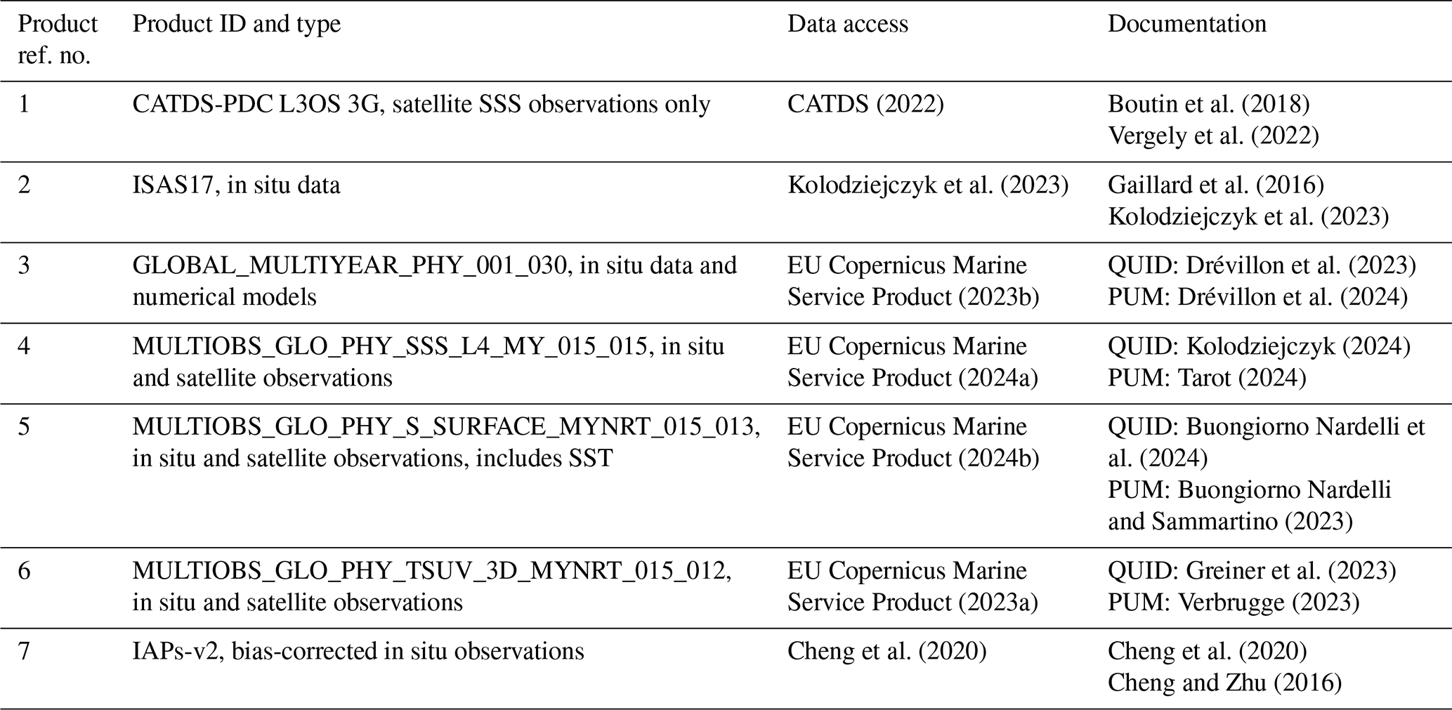
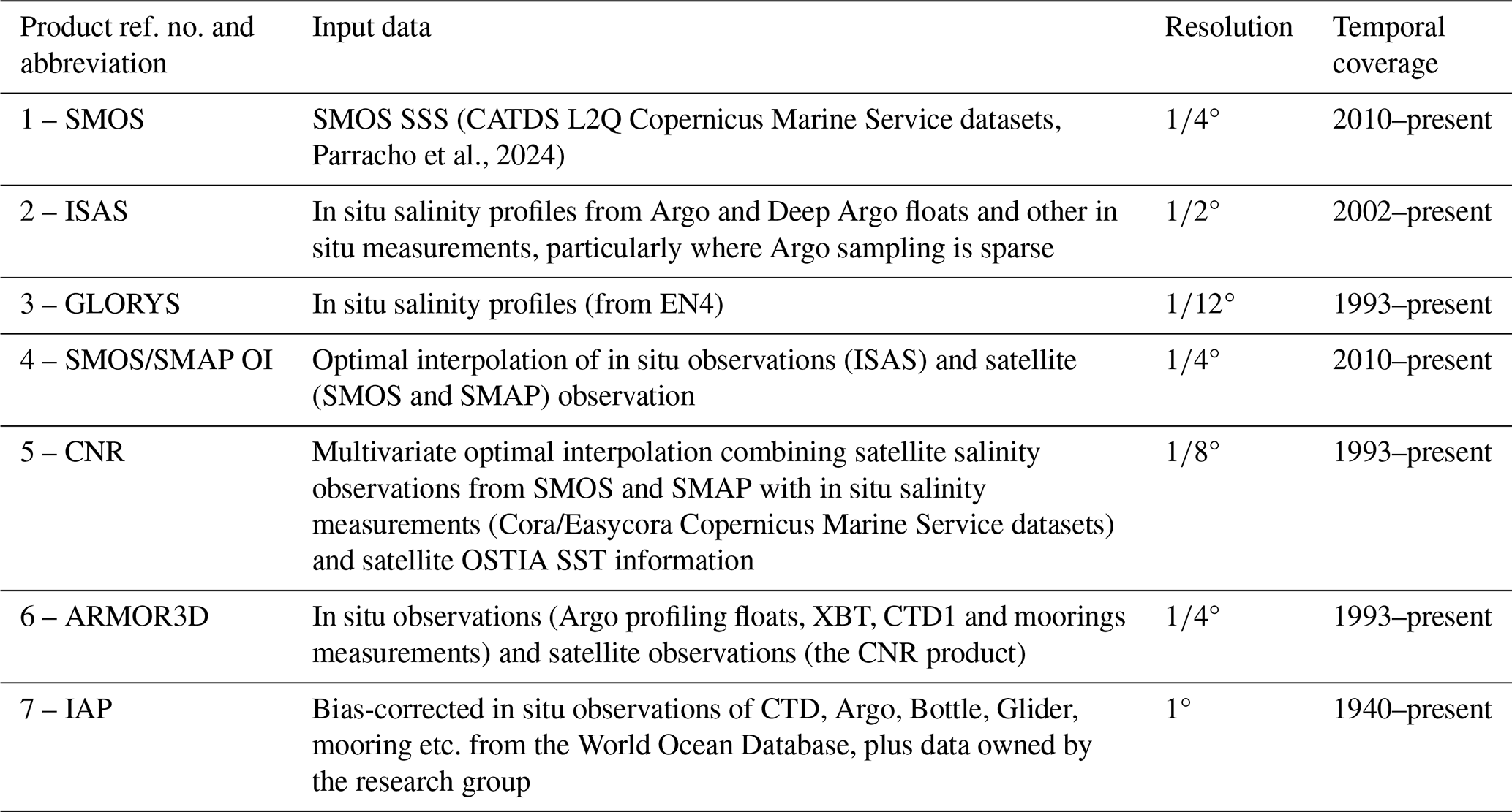
The number of SSS products is increasing thanks to the advances in satellite remote sensing of SSS. In this paper, we used SSS products yielded from different technologies: satellite-only, in situ-only, and a combination of both satellite and in situ data (also exploiting multivariate approaches). Table 1 summarizes the seven SSS products analyzed in this work, while Table 2 summarizes their input data, resolution and temporal coverage. Products 1–6 provide the core information used to derive trends over the last 15 years. It is important to note that among the included SSS products, some of them provide independent information about SSS temporal variability; for example, the interannual variability in SMOS SSS (product 1) is independent from any product using only in situ SSS measurements, such as ISAS (product 2) or GLORYS (product 3). At the same time, other products are not independent as they use some of the same data. For instance, the SMOS/SMAP OI (product 4) uses SMOS and ISAS data in their optimal interpolation, while the ARMOR3D (product 6) uses the CNR SSS dataset (product 5) in their upstream. In this context, “independent” is used in a relative sense, referring to differences in the underlying salinity data sources rather than to all auxiliary variables used in the processing chains.

Table 2 Input data, resolution and temporal coverage of the products used in the study.

To assess if the significant trends observed for the last 15 years are consistent with longer term trends, the Institute of Atmospheric Physics (IAP, product 7) global ocean salinity gridded product (Cheng, 2022), available from 1940 to present, was used. The trends and statistical significance were computed for the salinity at the surface, for different time periods: 1960–2024 (the full period of the dataset was not used as data for 1940–1959 reportedly has a large uncertainty), 2005–2024 (the Argo period) and 2011–2024 (the satellite period).

3 Methods

The trends were computed using the Theil-Sen method (Theil, 1950; Sen, 1968) on the monthly mean anomalies of each dataset. These anomalies were computed by removing the monthly climatology in each dataset (for the period 2011–2024) from the monthly mean data. The Theil-Sen method is a non-parametric statistic that computes the median slope of all the pairwise combinations of points. This method has been shown to be less sensitive to outliers in the data than the more commonly used least squares method (Parracho et al., 2018).

The significance of the trends was assessed using a modified Mann–Kendall test (Hamed and Rao, 1998), which is suitable for autocorrelated data. A significant trend is one that differs from zero at 95 % confidence.

4 Results

4.1 Intercomparison of results obtained from different Sea Surface Salinity global products

The global SSS trends are shown for the different products in Fig. 1. The areas where the trends are not statistically significant are masked with stippling. The latitudes are restricted to between 50° S and 50° N because there are well known issues in satellite data related to sea-ice contamination and lower sensitivity of the L-Band radiometric signal to SSS near the polar regions where SST is low (Reul et al., 2020; Xie et al., 2023) and there are fewer in situ data (Gabarró et al., 2023).

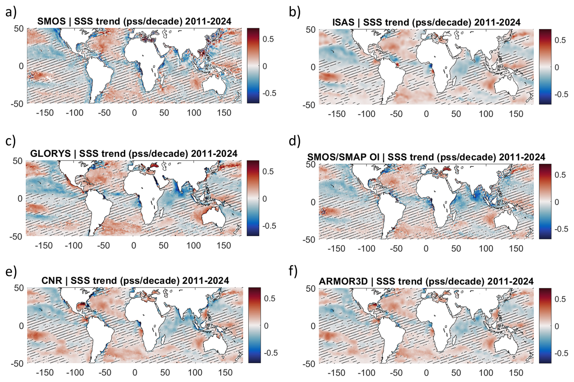
Figure 1 Linear trends (in pss per decade) in SSS computed using the Theil-Sen method for different SSS products: SMOS (a), ISAS (b), GLORYS (c), SMOS/SMAP OI (d), CNR (e) and ARMOR3D (f). Regions where the trends are not statistically significant using the Mann-Kendall test are covered by stippling.

In general, large areas of positive and negative statistically significant trends are found, and are consistent across the different analyzed SSS products. The agreement between the trends obtained with various products is particularly remarkable for datasets that are independent, such as SMOS (product 1) and GLORYS (product 3). We find similar results for these two datasets, especially away from the coast, and in regions where trends are statistically significant. Besides, consistent trends between SMOS/SMAP OI (product 4) and ISAS (product 2) are found, which can be partly explained by the fact that ISAS is used to constrain the large-scale variability of SMOS/SMAP OI. Some similarities between CNR (product 5) and ARMOR3D (product 6) trends are also expected, because CNR data is used as an upstream in ARMOR3D. The ARMOR3D and CNR products also include in situ observations (and weight them differently considering characteristic temperature decorrelation scales), therefore their trends are also close to ISAS and SMOS/SMAP OI. Slight differences are observed in the intensity of the trends, with slightly more intense trends found in SMOS and GLORYS data and slightly less intense trends in ISAS (e.g. in the North and South Atlantic). However, there are more regions of statistically significant trends in ISAS than in the other products, likely because the data is smoother. ISAS applies objective analysis with spatial and temporal smoothing to interpolate in-situ data, which reduces short-scale variability and results in a lower standard deviation. There are also differences between the products in smaller regions, such as river plumes (e.g. of the Amazon and Congo rivers),which are areas of higher variability. In the SMOS data, there are negative trends near the coast that are not present in the other datasets(e.g. in the Pacific near the coast of South America and in the Atlantic near the coast of South Africa). Whether this could be related to a temporal evolution of the SMOS land-sea contamination (Kolodziejczyk et al., 2016) remains to be further studied.Nevertheless, these negative trends appear on both ascending and descending SMOS passes (not shown) whereas SMOS land-sea contamination strongly varies between ascending and descending satellite passes. In addition, few in situ measurements are available near land and future studies would be needed to better assess trends there.

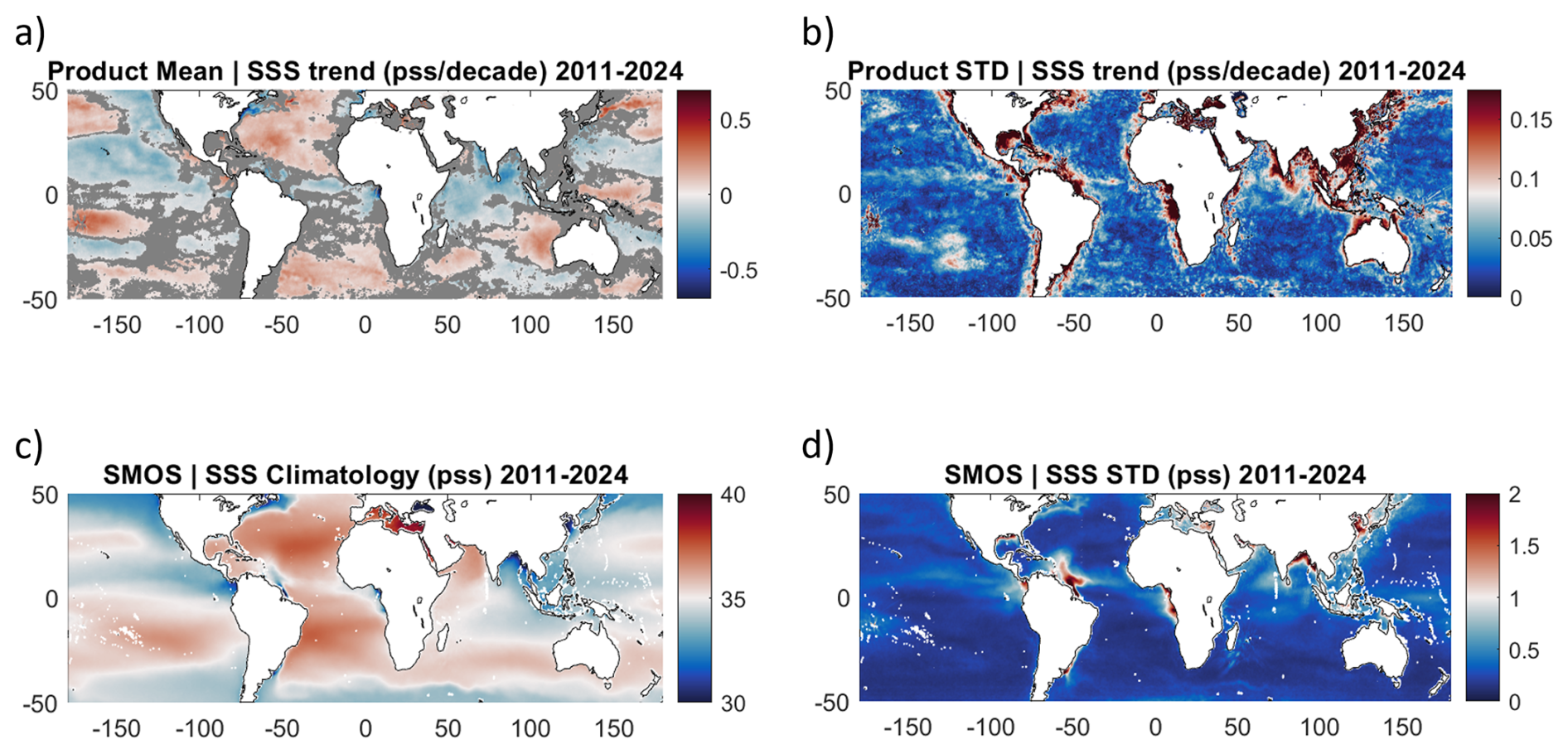
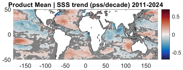
Figure 2 Mean trend (a) and standard deviation of the trends (b) in the products 1–6. The mean trend is overlaid with grey stippling for the gridpoints where the standard deviation of the trends exceeds the mean of the trends. Climatology (c) and standard deviation of SSS (d) for the SMOS dataset. The climatology and standard deviation maps for SMOS are consistent with the results obtained from the other datasets in the study (not shown).

In order to quantify the consistency between the trends derived from the different datasets, the mean value and standard deviation (SD) of SSS trends obtained from the 6 products were computed and are presented in Fig. 2a and b, respectively. The standard deviation (Fig. 2b) provides information about the level of uncertainty of the estimated trends, and the grid points where the standard deviation exceeds the trends were overlaid withgrey stippling over the mean trends in Fig. 2a. In general, the SD of the trends are about an order of magnitude smaller than the trends (under 0.05 pss per decade), which means that the trends derived by the different datasets are consistent with each other. However, there are some exceptions. The biggest SD in the trends obtained using the six datasets (Fig. 2b) corresponds to river plumes. For instance, in the Amazon River plume, ISAS shows a small area of positive trends (Fig. 1b) that is not observed in the other datasets, while ISAS, ARMOR3D and CNR show a positive trend in the Congo river plume that is negative in the observations-only datasets, SMOS and GLORYS. These river plumes are also regions of higher standard deviation of the monthly SSS (shown for SMOS in Fig. 2d). Some of the regions of higher SD of the trends also correspond to regions where the radio frequency interferences (RFI) contaminate the L-band radiometric signal, affecting the SMOS data. This is a local effect especially seen around Samoa, Barbados, and the Guinea Gulf (Bonjean et al., 2024).

In order to assess if the observed statistically significant trends correspond to an intensification of salinity patterns, as described in the literature and expected in theory, the trends in Fig. 2a were compared with the SSS climatology (Fig. 2c). We can see that some of the regions of higher salinity (e.g. the North Atlantic) also have positive SSS trends, while regions of lower salinity (e.g. the North Pacific) correspond to regions of negative trends. This reveals an increase in inter-basin contrasts. Other regions where “salty gets saltier and fresh gets fresher” are found in the Indian Ocean east of India (where a fresh region shows a freshening trend) and in the South Atlantic and west of Australia (where already saltier regions have a positive SSS trend).

Some regions, however, do not follow the intensification pattern. In the Southern Pacific Ocean there is a trend-dipole in a region of higher salinity, which closely resembles the patterns of SSS anomalies evolution observed and modelled during La Niña events (Fig. 4 in Hasson et al., 2014). In fact, during the period at study, there were three multi-year La Niña events (2010–2012, 2016–2018 and 2020–2023) which covered most of the investigated period and whose impact can be seen in the trends, with a negative SSS trend in the mid-latitudes in the Pacific and a positive SSS trend slightly south of the equator. Local deviations from simple water cycle amplification patterns are consistent with the results discussed in Buongiorno Nardelli and Iudicone (2025) and the trend dipole identified in the Southwestern Pacific matches the patterns shown in their Fig. S12, associated with the Central Pacific El Niño-Southern Oscillation mode. Both Pacific Decadal Oscillation (PDO) and El Niño Southern Oscillation (ENSO) modes can also explain the differences in the trends estimated for the Amazon plume during the different periods (and applying different techniques, in Buongiorno Nardelli and Iudicone, 2025).

To do an exhaustive analysis of the results obtained from the different products, the SSS variability in regions with statistically significant SSS trends is analyzed further in the next subsection.

4.2 Regions of important changes of Sea Surface Salinity

The regions where the linear trends in most SSS products are significant were delimited by the boxes shown in red in Fig. 3a (see the coordinates of the boxes in Table 3). The monthly time series of average SSS anomalies in each box are shown in Fig. 3b for the six different products and were used to compute the trends presented in Table 4 and Fig. 4, which shows the results for all products and regions. The trends' significance was tested, and non-significant trends are underlined.

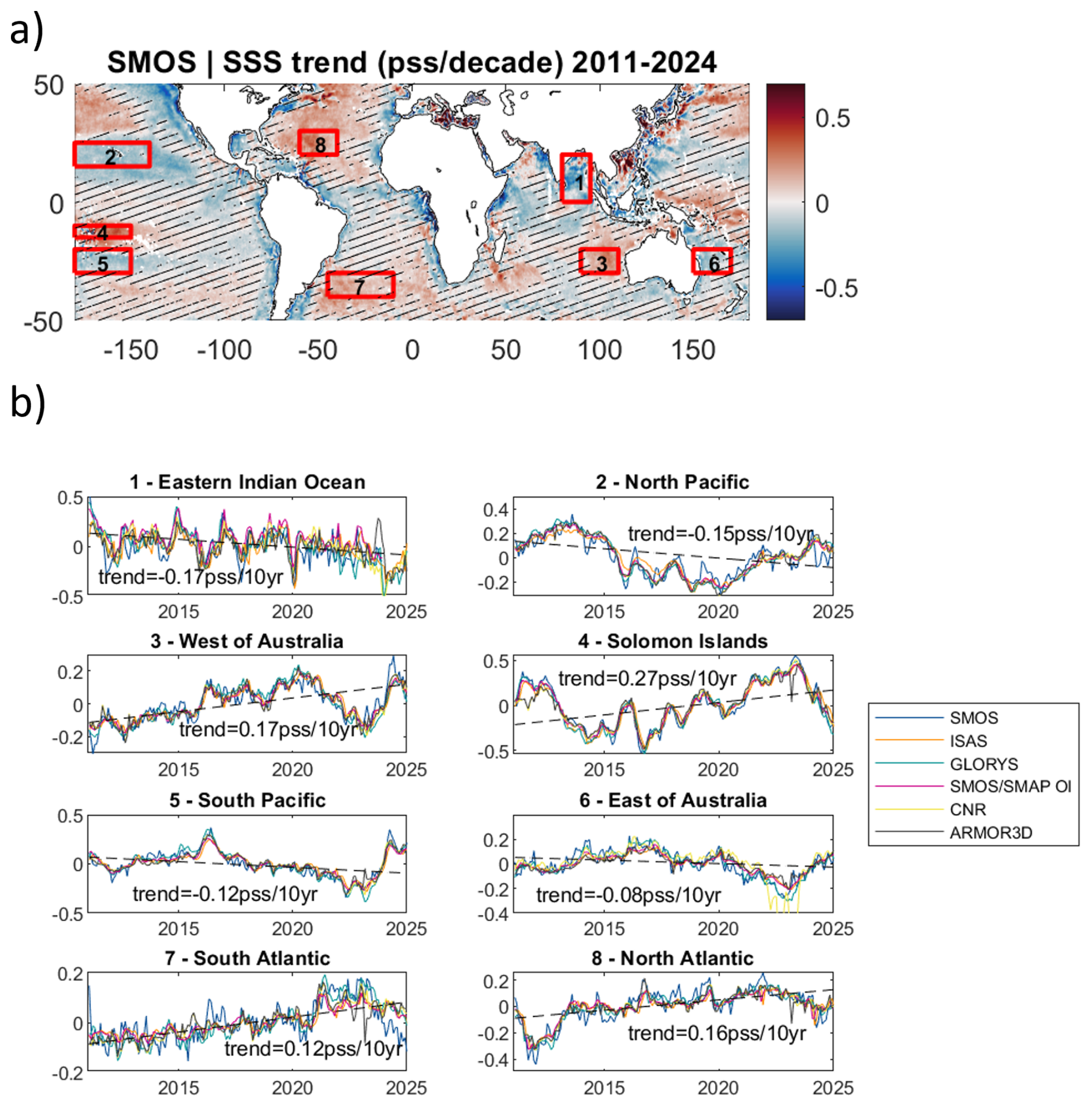
Figure 3 (a) Regions selected to depict the mean SSS anomalies time series and their trends are defined by the red rectangles and correspond to the regions where the trends are significant in most of the products. Regions are ordered according to their mean SSS in the regions, from the freshest region (1) to the saltiest region (8). (b) Time series of the SSS anomalies averaged over the regions selected in panel (a): 1 is the Eastern Indian Ocean, 2 is the North Pacific, 3 corresponds to West of Australia, 4 to region of the Solomon Islands, 5 to South Pacific, 6 to South Atlantic and 8 to North Atlantic. The mean trend across all products for each region is represented by the dashed line and indicated in each box.

Table 3 Coordinates of the red boxes defined in Fig. 3a.

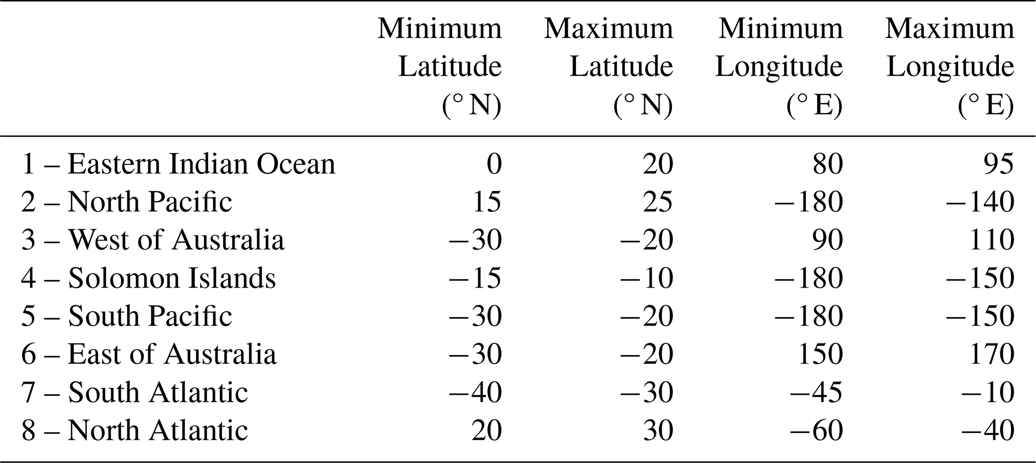
Table 4 SSS linear trends computed using the Theil-Sen method in the analysed regions (in pss per 10 years). Bold values are NOT significant (p-value > 0.05 in Mann-Kendall test).

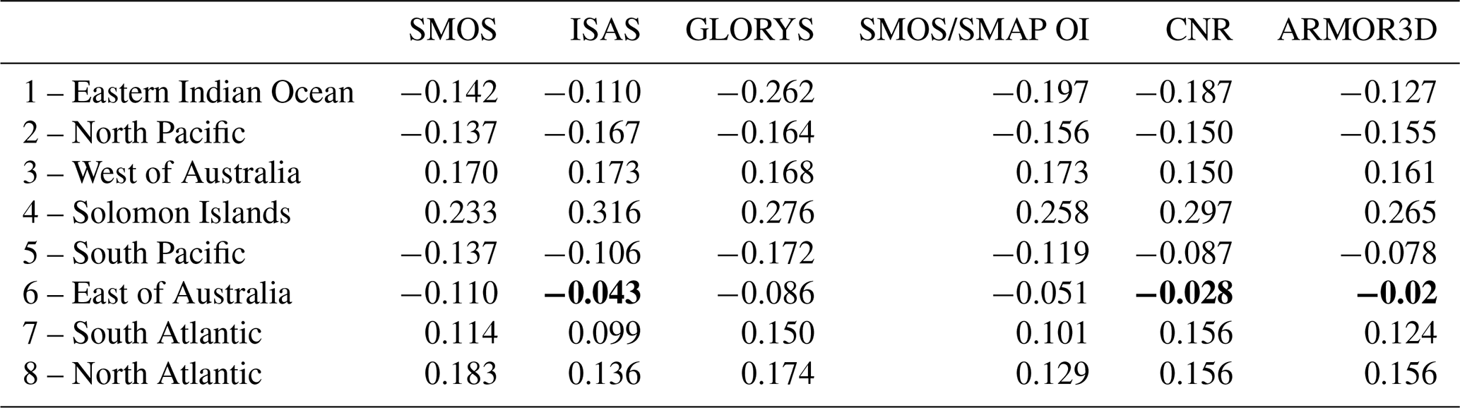
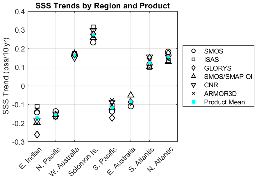
Figure 4 SSS trends computed using the Theil-Sen method in the selected regions, shown in Fig. 3a (in pss per 10 years) for all the data products, excluding the products where the trends are not statistically significant (p-value > 0.05 in Mann-Kendall test). Regions are ordered according to their mean SSS in the regions, from the freshest region on the left to the saltiest region on the right. The light blue dot corresponds to the mean trend across all products.

The time-series of the SSS anomalies of the 6 datasets in each of the 8 regions show a general good agreement among them, with different products superposing well (Fig. 3b).

In spite of the general good agreement between SSS products, some differences are observed between the time series from the various products (Fig. 3b). On the one hand, some datasets show slightly more variability in certain regions. For example, SMOS and GLORYS show higher variability in the eastern Indian Ocean, where sparse in situ coverage coincides with strong coastal signals linked to river discharge and surface currents that are well captured by SMOS (Akhil et al., 2020). Increased variability in these datasets is also found in stratified regions such as the South Pacific near the South Pacific Convergence Zone (SPCZ), likely reflecting differences in SSS representation. Whereas SMOS samples only the upper centimeter of the ocean and GLORYS represents an average over the top meter (effectively a surface measure), the other datasets are more strongly influenced by deeper in situ observations. In addition, the $\mathrm{1}/\mathrm{12}$° eddy-resolving resolution of GLORYS in the tropics may amplify variability, even at low frequencies, compared to lower-resolution or more strongly filtered products. Conversely, in the Solomon Islands region, the higher SMOS variability may also be related to RFI contamination (Bonjean et al., 2024).

On the other hand, some of the datasets differ from the others at certain periods of time. For instance, the CNR time series separates from the others in the Solomon Islands in 2011. ARMOR3D, based on CNR data, also follows this discrepancy (probably related to the number and treatment of in situ observations, and handling of the background field in their processing chains). In the East of Australia in the 2022–2023 period, the higher weight given to in situ observations in the CNR processing algorithm may enhance the representation of certain regional processes that are less evident in the other datasets. In this context, the stronger negative SSS anomalies observed in CNR SSS in 2022–2023 may be associated with precipitation variability affecting the western New Caledonia region and consequently the East of Australia area in that period (Blunden et al., 2023). ARMOR3D separates from the other time series in February 2023 in the Solomon Islands, the South Atlantic, the North Atlantic, and the Eastern Indian Ocean. This is because of spurious data that should have been flagged and not used in the ARMOR3D near real time (NRT) data that was used to complete the reprocessed time series in the last 2 years of the study. In the Eastern Indian Ocean, there is no SMOS or SMOS/SMAP OI data from December 2023, due to RFI contamination in the satellite data in the region. Finally, SMOS separates from the rest of the time series in the South Atlantic after 2024 for an unclear reason.

For all the datasets, some regions show a clear interannual variability, such as in the North Pacific and the Solomon Islands that can affect the result of the linear trend algorithm. Nevertheless, the statistically significant trends in these regions indicate a robust long-term change despite interannual variability. In general, according to Table 4 and Fig. 4, the trends are statistically significant in these boxes across all datasets, with the exception of East of Australia in the ISAS, CNR and ARMOR3D datasets, with statistically significant trends having the same sign and order of magnitude in most datasets. In the studied regions, the trends obtained for the climatological fresher regions are negative, but not all the trends of the climatological saltier regions are positive, with negative trends obtained in the South Pacific and East of Australia. Finally, the Eastern Indian Ocean is the region where the trends vary the most from one product to another (between −0.110 pss per decade in ISAS and −0.262 pss per decade in GLORYS, Table 4).

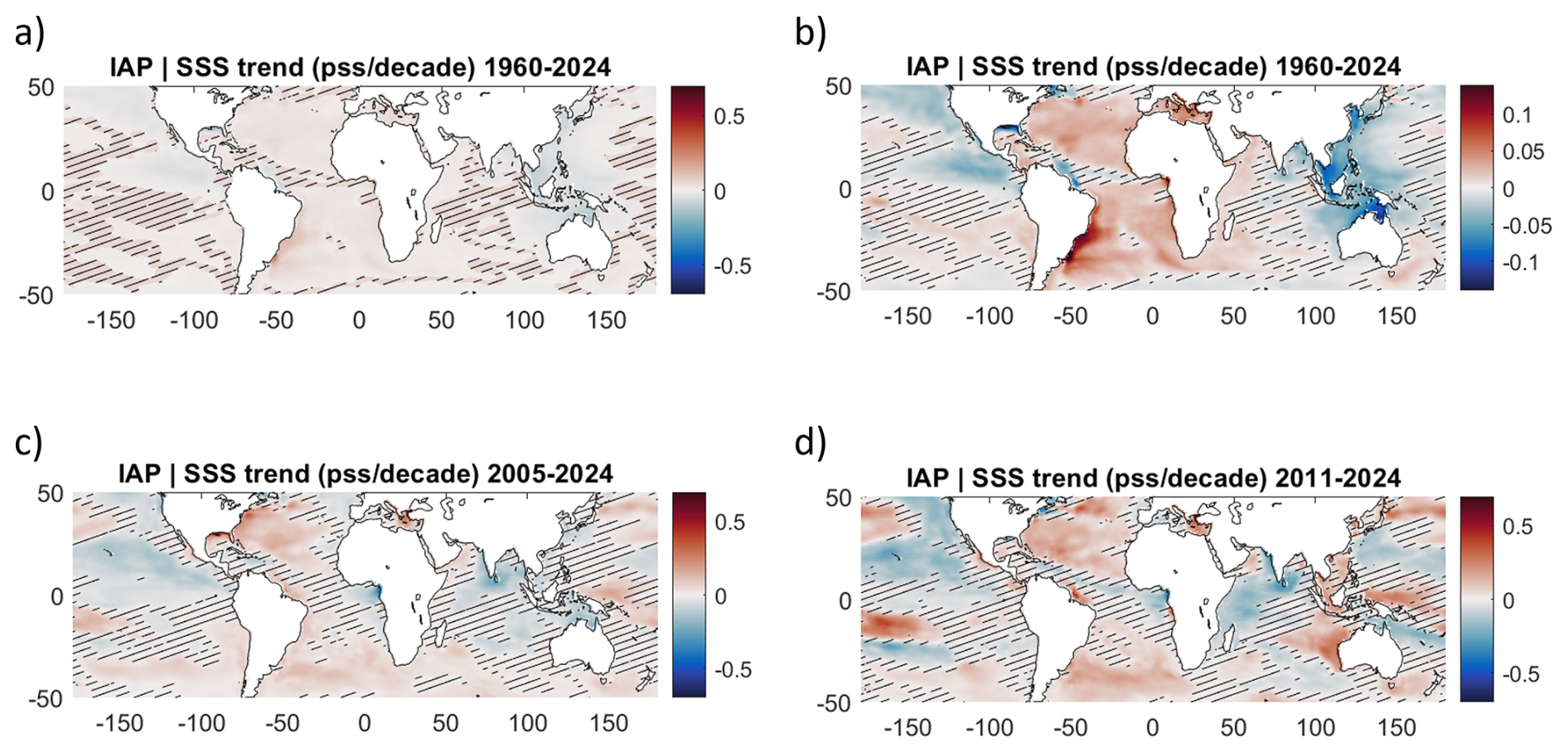
Figure 5 Linear trends in SSS computed using the Theil-Sen method for the IAP product at different periods of time. The regions where the trends are not statistically significant according to the Mann-Kendal test are covered with stippling. The top panels (a) and (b) correspond to the trends for the 1960–2024 period. They show the same trends with different colorscales. The bottom panel includes the trends for the 2005–2024 (c) and 2011–2024 (d) periods. The colorscales in panels (a), (c) and (d) are the same, for easier comparison of the order of magnitude of the trends for different time periods, while the colorscale in panel (b) is adjusted to better visualize the less intense trends for 1960–2024.

4.3 Comparison with long term SSS trends

The IAP product was used to assess if the results for the last 15 years are consistent with longer term trends. For the satellite period (2011–2024), the trends obtained in the IAP dataset are consistent with the ones obtained in the other datasets (compare Fig. 2a with Fig. 5d), and the same regions of significant positive and negative trends were found. However, when the period is extended to the Argo period, the trends are less intense (by a factor of 2) and although most regions show a trend of the same sign as the sign of the trends estimated for the satellite period, there are also some differences (e.g. west of Australia). For the longer 1960–2024 period, the trends have an intensity that is even lower than the trends observed for the satellite period by a factor of 5. Moreover, the longer-term trends (Fig. 5a and b) show a pattern very similar to the SSS climatology shown in Fig. 2c (as expected from the literature). These results suggest an intensification of the SSS trends in the last 15 years or could also be due to the scarcity of observations in the pre-Argo period that lead the gridded observations to be too constrained by (and tend more towards) the climatology. In addition, when looking at such a short period as 15 years, interannual and interdecadal variability have a strong influence on the estimation of a linear trend (as seen in the time series of Fig. 3b), and notably, the 2011–2023 period featured the strongest and longest La Niña events since 1980.

In fact, short-term trends can be very affected by internal variability, whereas long-term trends are slowly emerging. By comparing the trends obtained at different time scales we can begin to separate anthropogenic trends from natural variability. In this sense, Fig. 5 highlights that the short-term trends in some regions are consistent with the longer-term trends, most notably the increase in the interbasin contrast, with the increasing salinity trend in the North Atlantic and a decreasing salinity trend in the North Pacific. Short-term trends are also consistent with long-term trends in the increasing salinity of the South Atlantic and freshening Indian ocean off the coast of India. These results agree with an anthropogenic modification of the Hadley cell (Gulev et al., 2021; Pinho et al., 2021) and the long period of negative-phase Pacific Decadal Oscillation (PDO) in the years at study (Sun et al., 2022), as also suggested in Buongiorno Nardelli and Iudicone (2025). Other past studies (e.g. Wills et al., 2018) have also found it difficult to separate global warming from PDO and ENSO.

5 Conclusions

Whereas several papers have already examined long-term salinity trends using in-situ datasets, the novelty of this paper lies in the use of two independent sources of data to compute SSS trends over the past 15 years: up-to-date products derived from satellite data on one hand, and from in situ data on the other hand. Satellite data offer spatial and temporal coverage of SSS that was previously unattainable, and the length of the satellite record is now becoming sufficient for deriving statistically significant trends. In this paper, we analyzed various products from different datasets and found consistent trends, even when comparing independent datasets such as SMOS (a satellite-only dataset) and GLORYS (a model reanalysis which assimilates only in situ salinity and other in situ and satellite parameters).

Past studies have shown that spatial patterns of salinity change over multiple decades generally resemble the average salinity fields. However, those earlier studies referred to the period from roughly 1950 to 2008 (i.e., the pre-Argo era), when observations were sparse. In contrast, our analysis covers the period from 2011 to the present and identifies several regions where the trends do not follow the pattern of the climatology. This suggests local deviations from simple water cycle amplification patterns. This was also found, for example, by Vinogradova and Ponte (2017) for the period between 1993 and 2010, which they explained by the fact that anthropogenic hydrological signals take longer to emerge in the sea surface salinity compared to the surface freshwater fluxes. Indeed, comparison of our results with a long-term dataset derived from a combination of in situ observations and model outputs reveals consistent trends between the datasets over the past 15 years; however, these patterns differ from the longer-term trends. On the one hand, a comparison with the trends in this dataset for the Argo period (post-2005) showed that the intensity of trends has increased in recent years (although there can also be salinity sensors drift in the Argo data; Wong et al., 2020). While, on the other hand, a comparison with the longer-term trends (1960 to present) allowed us to separate trends that are part of long-term trends (such as the positive trend in the North Atlantic, which is a common feature of all periods and products), from the trends resulting from natural variability (such as the positive and negative trend pattern found in the Tropical Pacific due to the predominance of weak to strong La Niña conditions during the 2011–2024 period).

This study has shown that satellite, in situ and reanalysis SSS trends agree well in most regions (although longer records are still necessary to further minimize the influence of interannual and interdecadal variability), suggesting that these different SSS datasets could be used in the future to derive an SSS Ocean Monitoring Indicator.