Three decades of marine bioregions evolution through analysis of phytoplankton phenology

Ocean biogeochemistry is undergoing significant modification in response to climate change. To better track these evolutions, we present a novel ocean monitoring indicator that follows the temporal evolution of marine bioregions of similar phytoplankton phenologies. Chlorophyll a concentration observations from remotely sensed ocean color describe seven distinct marine bioregions characterized by their unique patterns of phytoplankton biomass seasonality. The sizes and locations of these bioregions are monitored from 1998 to 2024 using a multi-sensor merged L4 ocean color product. While the bioregions' extents appear to follow interannual and decadal climate variability, their long term evolution suggests a poleward extension of less seasonal phytoplankton phenology, which is generally characteristic of the tropical and subtropical bands. This innovative approach allows the systematic monitoring of how phytoplankton adapt their seasonal cycle in response to changes in environmental conditions, hence giving valuable insights into the evolution of marine ecosystems over the past three decades and helping advance our understanding of global ocean biological responses to environmental change.

1 Introduction

Phytoplankton, the main primary producers in the ocean, sustain marine food webs (Fenchel, 1988; Kiørboe, 1993) and play a central role in regulating oceanic carbon fluxes (Falkowski, 1994). Environmental conditions shape phytoplankton growth and losses through “bottom-up” (e.g., light and nutrients availability) and “top-down” (e.g., grazing) processes. Over the past three decades, satellite ocean color measurements make it possible to estimate phytoplankton biomass (Behrenfeld et al., 2005) proxied by chlorophyll a concentration (Huot et al., 2007). This, in turn, has enabled the study of phytoplankton phenology (i.e. the temporal succession of main biological events) (Longhurst, 2007; Racault et al., 2012; Sapiano et al., 2012; Boyce et al., 2017). Climate influences the distribution of environmental factors that, in turn, regulate the spatiotemporal dynamics of phytoplankton biomass (Falkowski and Oliver, 2007). Distinct seasonal patterns emerge along latitudinal gradients, from the equator to the poles (Longhurst, 1995). At high latitudes, primary production is mainly light limited, whereas in tropical and subtropical regions, phytoplankton production is essentially nutrient limited (Boyce et al., 2017). Like the marine environment itself, phytoplankton biomass responds to both annual and decadal climate variability (Li et al., 2024).

Table 1 Product table.

Climate change is altering oceanic ecosystems (see OSR10 Chap. 1.3 by Lévy et al.), with complex impacts on phytoplankton growth. For instance, rising sea temperatures might directly affect metabolism (O'Connor et al., 2009) but also environmental conditions through enhanced water column stratification (Yamaguchi and Suga, 2019), which in turn might further limit growth by hindering upward transport of nutrients to the sunlit layers (Sarmiento et al., 2004; Fernández-González et al., 2022). As for terrestrial plants (Cleland et al., 2007; Inouye, 2022), marine phytoplankton are expected to respond to these environmental changes by adjusting their seasonal cycles (Winder and Sommer, 2012). Most of the documentation effort focused on variations in the onset, duration, and intensity of bloom events (e.g., Sommer and Lengfellner, 2008; Martinez et al., 2011; Henson et al., 2018; Salgado-Hernanz et al., 2019). These changes may cause phenological mismatches hence disrupting energy transfer to higher trophic levels (Visser and Both, 2005; Asch et al., 2019) and have broader implications for the global carbon cycle (Fisher et al., 2025). Consequently, establishing robust indicators monitoring interannual to decadal changes in phytoplankton phenology is critical to better address the evolution of the marine ecosystem with climate change.

With the large amount of remotely sensed ocean color observations, numerical clustering methods emerged as key tools to identify regions with similar seasonal dynamics of phytoplankton (hereafter referred to as bioregions) (International Ocean Color Coordinating Group; IOCCG et al., 2009). Several studies (e.g. D'Ortenzio and Ribera d'Alcalà, 2009; Lacour et al., 2015; Ardyna et al., 2017; Boyer et al., 2017; Kheireddine et al., 2021; Baudena et al., 2025) have applied such methods to partition oceanic domains into bioregions characterized by similar seasonal patterns of chlorophyll a concentration, which are often used as a basis for inferring provinces of similar biogeochemical functioning. Similarly to how Mayot et al. (2016) extended D'Ortenzio and Ribera d'Alcalà (2009) climatological partitioning of the Mediterranean Sea, this study presents an ocean monitoring approach built on Baudena et al. (2025) climatological bioregionalization of the global ocean. This method tracks variations in the extension of the bioregions in respect of time to reveal the trends in geographical changes of phytoplankton phenology. The main idea behind our approach is that tracking these variations may serve as a relevant proxy for assessing changes of phytoplankton dynamics, which, in turn, could inform on main variations of environmental factors of the marine ecosystem.

We introduce here a proof of concept for such an approach using the supervised clustering method introduced in Baudena et al. (2025). Annual partition of the global ocean (56° S–56° N) from 1998 to 2024 is obtained by classifying annual time series of remotely sensed chlorophyll a concentration (Copernicus-GlobColor) into bioregions. After presenting the mean climatological state of the bioregions, we investigate their change in surface area over the last three decades. Then, building on D'Ortenzio et al. (2012) and adapting methods from Higgins et al. (2016), originally applied to terrestrial biomes, we compare the geographical extension of the bioregions between two decadal periods at the greatest extent of our dataset, (1998–2007 and 2015–2024) to identify the main trends in the reorganization of phytoplankton phenology. Finally, possible correlation with environmental changes and method limitations are evoked in the discussion section.

2 Material and methods

2.1 Data

Chlorophyll a concentrations data were retrieved from the merged multi-sensor ocean color product ref. no. 1 (see Table 1). This product offers cloud free remotely sensed surface chlorophyll a concentration at a 4 km spatial resolution and daily intervals. Using such a L4 product (an optimally interpolated, merged satellite dataset), as compared to L3 (merged product) in Baudena et al. (2025), compensates for the lack of observation inherent to satellite ocean color (Stock et al., 2020) and ensures a maximal spatialization of the bioregions at an annual temporal resolution.

2.2 Supervised Clustering

Annual ensembles of seasonal time series of chlorophyll a concentration were built from 1998 to 2024. The time series composing them were all processed similarly to allow subsequent classification according to Baudena et al. (2025) supervised clustering method. In short, within each annual ensemble, each individual time series characterizes the seasonal evolution of chlorophyll a concentration over a 1° × 1° grid. Following the method detailed in Sect. S1 in the Supplement, the time series were obtained averaging all available observations within each 1 × 1° pixel over a 8 d temporal window. To dampen sub-seasonal variations, time series were all smoothed with a 5 weeks centered rolling average method. Finally, all annual time series were normalized by their maximum to ensure that the clustering method focuses on their shape rather than on their magnitude.

Time series associated with pixels in the Arctic and Southern Oceans (respectively above 56° N and below 56° S) were removed from every annual ensemble due to lack of continuous satellite observation through winter in relation to permanent cloud presence and polar night. Coastal pixels located within 111 km (∼ 1°) from the coast were also discarded due to the uncertainty in chlorophyll a concentration estimations within optically complex waters (Case 2 waters). As a result 80 % of the global ocean area is considered. In the southern hemisphere, time series were all shifted six months backward, to ensure identical sequencing of seasons in the time series of all pixels.

Each annual ensemble was then partitioned into the seven clusters of Baudena et al. (2025) based on their seasonality patterns. These seven clusters were found to optimally partition open ocean seasonal cycles of surface chlorophyll a concentration in respect of multiple statistical tests discussed in the companion study. The assignment of a given time serie into one of the clusters was done according to its minimal euclidean distance (maximal similarity) with the central time series of Baudena et al. (2025) clusters. To prevent assignment of too dissimilar seasonal patterns, a threshold distance was considered to accept (distance below the threshold) or refuse (distance above the threshold) an assignment. To account for the method's sensitivity to this hyperparameter, we discretized a range of possible values, defined by the minimum and maximum classification distances found among the most deviating elements of any cluster, from 1.33 (cluster 1) to 2.60 (cluster 7), based on the unsupervised clustering of Baudena et al. (2025). Each annual ensemble was partitioned several times from a low (strict definition of the clusters) to high threshold values (lax definition of the clusters) selected within this range with a regular step of 0.05 (see sensitivity analysis in Sect. S2). At least 88 % of the time series were always successfully sorted within the seven clusters (see Fig. S2b). Unclassified time series, mostly located in regions of low satellite data availability region (see Fig. S2a), were all excluded from ulterior analysis.

2.3 Bioregions

The spatial projection of each pixel's membership over the global ocean forms large coherent spatial domains similarly classified. These oceanic domains correspond to the bioregions as defined by Baudena et al. (2025). As a reminder, bioregions share similar seasonal patterns in phytoplankton phenology suggesting a common biogeochemical functioning (Longhurst, 1995). Over time, the spatial definition of the bioregion might change with annual time series characteristic of a given pixel being attributed to different clusters over different years. A change of phytoplankton phenology is attributed to a pixel when its bioregion changes from one year to another. For a given pixel, the frequency of phenology change is defined as the total sum of these changes over the study period. These changes might present oscillating patterns from annual to decadal period or long term trends.

Three climatological partitions of the global ocean were considered hereafter. They were constructed by keeping, in each pixel, the most frequent bioregion over the selected temporal extent. The three considered periods are: from 1998 to 2024 and two decadal periods from 1998 to 2007 and from 2015 to 2024. The former climatological period supports the documentation of the average bioregion extent while the latter two decadals periods were chosen at the edge of the temporal span to support the documentation of long term changes in the bioregion's extent. The use of decadal bioregions also dampens interannual variability.

When comparing the decadal bioregions' extent between the 1998–2007 and the 2015–2024, we attribute a stable phenology change to a given pixel when its classification changed between the two periods and if this assignment remained identical for more than six years in each of the two decades. This temporal criterion was chosen strictly above half a decade to grant a reasonable and robust indicator of the bioregion persistence while remaining permissive in respect of inter annual climate variability.

To assess phytoplanktonic biomass across the bioregions, we analyzed their chlorophyll a concentrations, presented as probability distribution functions in Fig. 1b. The distribution for bioregion 1 is notably bimodal, showing a minor peak near 0.03 mg m⁻³ and a dominant one just above 0.1 mg m⁻³. This finding prompted us to subdivide bioregion 1, after the clustering, based on a threshold of 0.06 mg m⁻³ for yearly average chlorophyll a, creating an oligotrophic group (below the threshold) and a mesotrophic group (above the threshold). Although both sub-regions exhibit a similar non-seasonal pattern, this subdivision reveals distinct phenologies, suggesting they are controlled by different environmental forcings that either sustain or inhibit year-round phytoplankton growth.

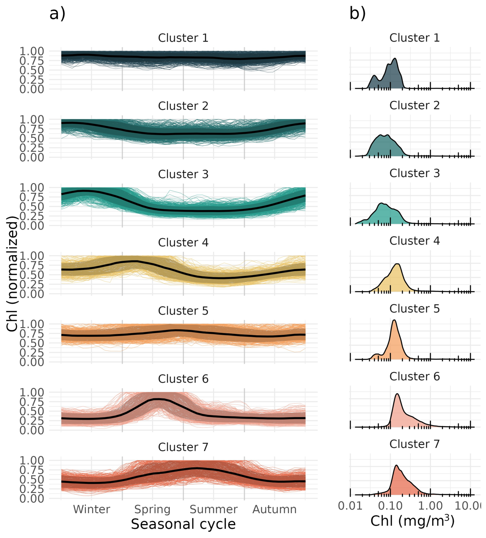
Figure 1 Clusters resulting from the supervised clustering of the ensemble of year 2024 from product ref. no. 1 according to the strictest threshold. The left panel (a) shows the mean normalized seasonal cycles within each cluster (thick continuous black line) within its 10 % and 90 % percentiles (transparent black bands). In the background, examples of time series within that cluster are represented. The right panel (b), displays the distribution of chlorophyll concentration within each cluster.

2.4 Uncertainties estimation

Following the set of threshold distance, each annual ensemble is partitioned twenty six times (see Sect. 2.2). In each of these partitions, the distribution of the bioregion surface area relative to the set of threshold distances is characterised hereafter by its central value (the median) within its interquartile range (Q1–Q3). The interquartile range of surface area estimates accounts for the bioregionalization method uncertainty. All surface areas are reported relative to the total global ocean area. To identify long-term changes, we fitted a linear model to the central surface area estimates in respect of time. The statistical significance of these linear trends was determined using a Spearman rank correlation, with a trend considered significant at p < 0.1.

3 Results

Our analysis is presented in three parts. First, we recall the phytoplankton phenology and climatological repartition of the seven marine bioregions (described in more details in Baudena et al., 2025). Second, we assess the interannual variability and long-term trends in the surface area evolution of each bioregion from 1998 to 2024. Finally, we identify the locations of stable phenological changes by comparing two distinct decades at the edges of the period.

3.1 Bioregion and phytoplankton phenology

For each year, the supervised clustering method subdivides the ensemble into the seven clusters identified in Baudena et al. (2025). These clusters outline specific phenological patterns inferred from the mean seasonal cycle of chlorophyll a concentration (Fig. 1a). These patterns, corresponding to the bioregions in Fig. 2a, range from no clear seasonality (bioregion 1) to those with pronounced single or double peak events (bioregions 7–6–4), which are typical of blooms in temperate and high-latitude systems, as we found in Fig. 2a.

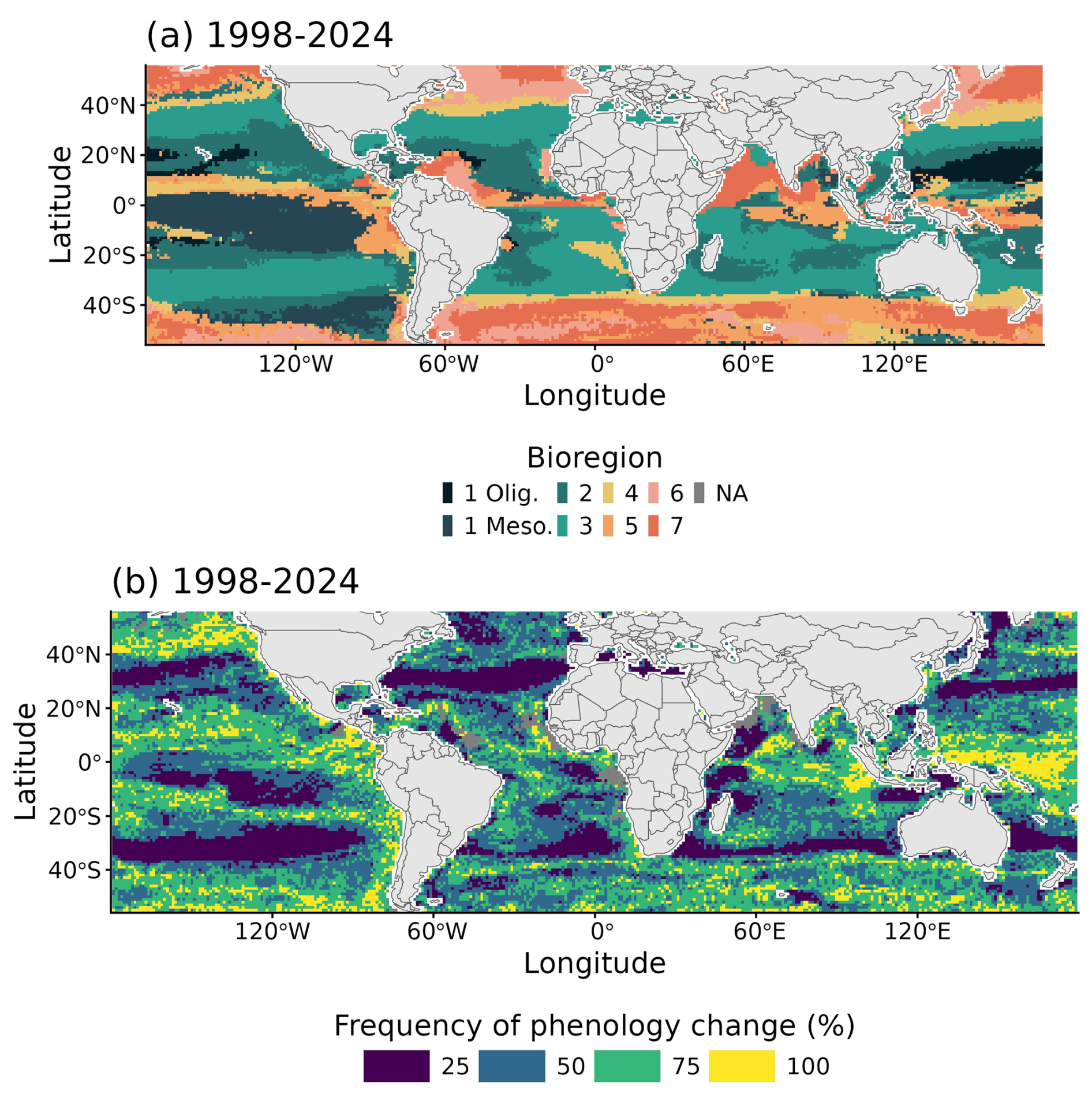
Figure 2 (a) Climatological distribution of the bioregions in the 1998–2024 period. (b) Amount of phenology change per pixel over the 1998–2024 period given in % of the total number of considered years. Both panels display the results obtained using the least strict clustering criteria on the ensemble processed from product ref. no. 1. Pixels designated as NA (in grey) refer to the position of the time series that were not successfully classified.

In agreement with Baudena et al. (2025), the climatological distribution of the related bioregions over the 1998–2024 period (Fig. 2a) follows a meridional distribution sketching coherent, large-scale structures corresponding to major oceanic domains, such as the subtropical gyres (bioregions 1 Olig., 2 and 3) and convergences zones (bioregion 4). The biogeochemical relevance of this partitioning is reinforced by the distribution of chlorophyll a concentrations within each bioregion (Fig. 1b). A clear poleward productivity gradient emerges, with the lowest surface biomass in the perpetually stratified regimes of the subtropical band and the highest in the high-latitude bloom regions (bioregion 6–7). This aligns with established knowledge of global ocean productivity patterns (Behrenfeld et al., 2005).

Baudena et al. (2025) offered a biogeochemical interpretation of the bioregions, summarized as follows. Bioregions 6 and 7 correspond to Longhurst (1995)'s model 1 (polar, irradiance-limited). Bioregion 5 exhibits features of both model 1 and model 2 (mid-latitude, nutrient-limited spring production peak). Bioregion 4 closely aligns with the Bloom bioregion identified by D'Ortenzio et al. (2012). Bioregion 3 matches Longhurst (1995)'s model 3 (subtropical, winter nutrient-limited), whereas Bioregion 2 closely resembles the Tropical bioregion described by D'Ortenzio et al. (2012). Finally, Bioregion 1 corresponds to Longhurst's model 4 (tropical). Its additional subdivision, introduced here, produces spatially coherent domains that distinguish between oligotrophic regions in the centers of subtropical gyres and mesotrophic regions primarily distributed around the equator.

3.2 Temporal evolution of the bioregions

The boundaries of bioregions in Fig. 2a are not static. Figure 2b displays the frequency of changes in each pixel bioregion's affiliation, interpreted as changes in phytoplankton phenology, over the 1998–2024 period. These changes occur most frequently in transitional areas in-between major bioregions, as well as in coastal zones, over the equatorial band, and over high-latitude regions of the northern Pacific and Southern Ocean (Fig. 2b). Bioregion 3, centered at 30° in both hemispheres, appears as the most stable bioregion.

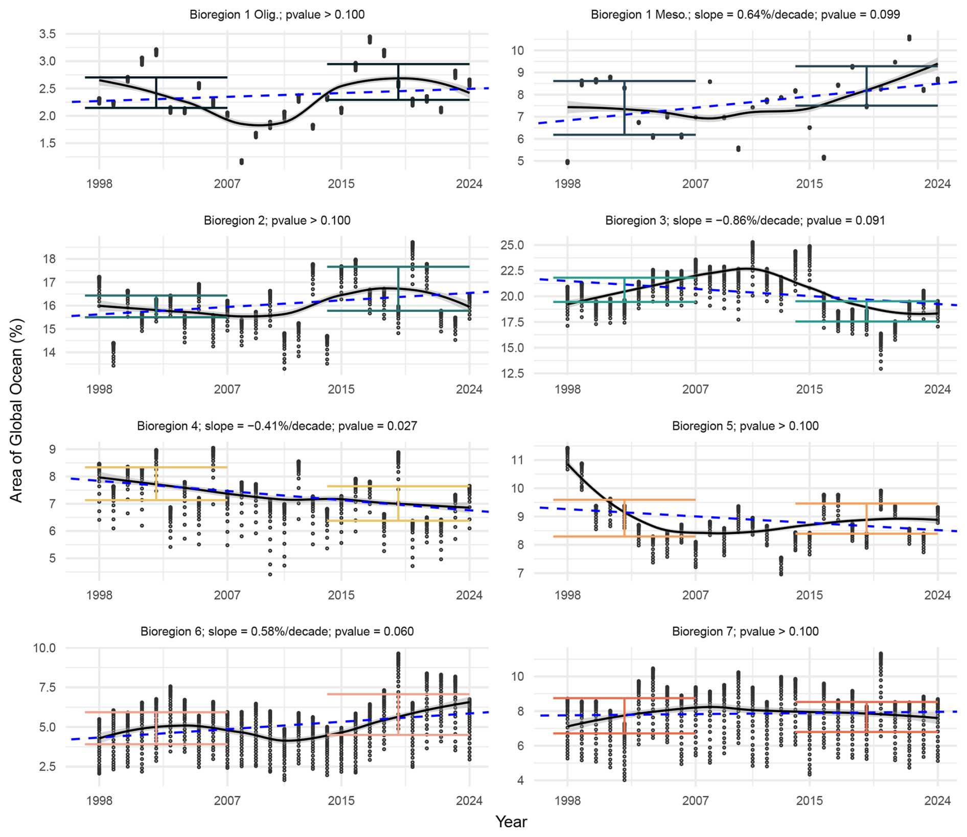
Figure 3 Evolution of bioregions' surface area from 1998 to 2024. The time evolution of black dots represent estimates of the areas following the varying acceptance thresholds. The black trend line displays the smoothed centered 10-year rolling average, the blue dotted line corresponds to the linear tendency of the annual median area estimate. Panels' titles show the linear trends on the condition that it was found significant (p < 0.1). First and third quartiles of the decadal bioregions (1998–2007 and 2015–2024) are indicated as colored error bars. Note the varying y-scale across panels.

A visual analysis of the temporal evolution of each bioregion's surface area (Fig. 3) reveals strong interannual variabilities (time evolution of black dots) in all bioregions. Bioregions 1, 2, 3 and 6 also display high decadal variability (black lines). Linear trend analysis (p < 0.1) indicates a significant reduction in the global surface area of bioregion 3 and bioregion 4. Conversely, the mesotrophic bioregion 1 shows a significant expansion. While surface areas of bioregions 6 and 7 exhibit large changes from one year to the other, their surface area estimates are associated with large method uncertainties (∼ 50 %), precluding the consideration of the trend significance.

3.3 Stable changes of phenology

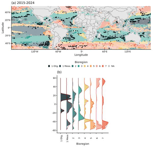
To isolate long-term trends from interannual variability, we identified areas with stable phenological changes between the 1998–2007 and 2015–2024 decadal periods. As highlighted in Fig. 4a, these regions are mostly located within the tropical and subtropical band. Overall 4.93 % [4.56 %, 5.06 %] of the global ocean is affected suggesting slow transitions in essentially steady conditions. The dominant pathways in phenology transition are summarized in Table 2. The most prominent change (1.82 % of the global ocean) is the transition from bioregion 3 to the less seasonal bioregion 2, occurring primarily in the subtropical Pacific and Indian Oceans. Other significant shifts include the expansions at lower latitude of bioregion 1 at the expense of bioregion 2 (0.62 %) and of bioregion 3 at the expense of bioregion 4 (0.27 %). In the North Atlantic's temperate band, a notable net transition from bioregion 7 to 6 also occurred (0.09 %). As summarized by Fig. 4b, the most prominent trend is a poleward expansion of bioregions of weaker seasonality. These spatial patterns of change correspond to the surface area trends observed over the full time series (Fig. 3).

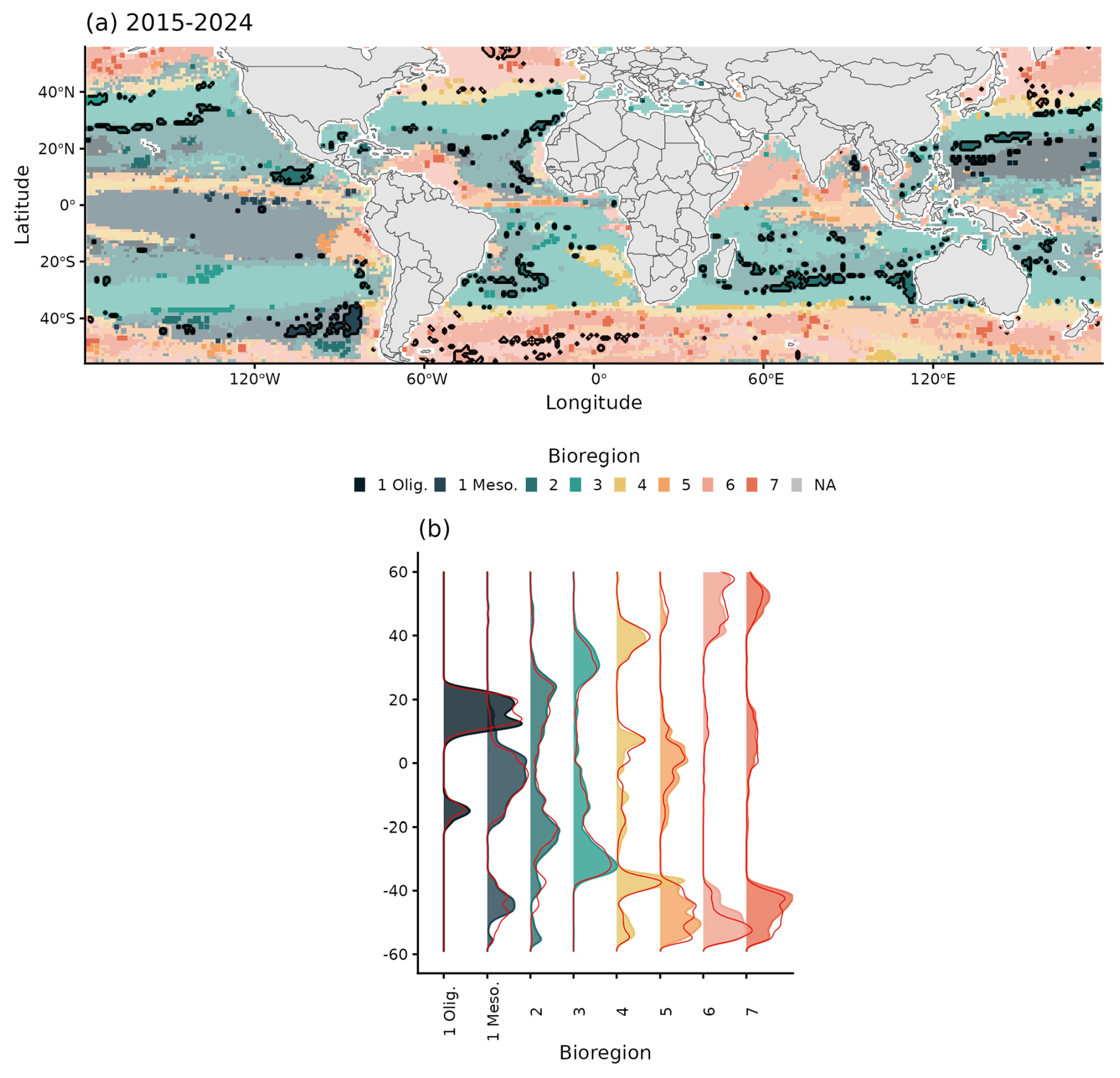
Figure 4 (a) Bioregions in the 2015–2024 decadal period with stable changes identified by black contours. (b) Latitudinal distribution of bioregions for the 2015–2024 decadal period (filled), compared with the 1998–2007 decadal period (red line).

Table 2 Major pathways among stable phenology changes. Changes in surface area from one bioregion to another are given relatively to the global ocean. Estimates are given within their first and third quartiles and grouped by oceanographic basins. Minor changes, associated with an area inferior to 0.01 % of the global ocean, are not represented. Estimates highlighted in bold indicate values greater than 0.1 % of the global ocean.

4 Discussion and conclusion

Our analysis introduces a novel ocean indicator approach that distinguishes between intermittent, year-to-year variability and persistent, long-term shifts in phytoplankton phenology. While boundary regions exhibit frequent intermittent changes (Fig. 2b), our decadal analysis finds that nearly 5 % (see Table 2) of the global ocean experienced a displacement of phytoplankton phenology suggesting persistent ecosystem reorganization over the past three decades. The cascading changes (i.e., transitions from bioregion 4 to 3, bioregion 3 to 2, and 2 to 1) identified above, are possibly driven by an intensification of upper-ocean stratification in relation to climate warming (Capotondi et al., 2012). At these low latitudes (30° S–30° N), a shallower vertical mixing prevents entrainment of deeper nutrients (Vereshchaka and Shatravin, 2025) therefore hindering biomass accumulation of surface waters (Sarmiento et al., 2004; Polovina et al., 2008). The robustness of our ocean indicator approach is further validated in the temperate North Atlantic, where despite high method uncertainties, the documented shift from a double to a single bloom phenology (bioregion 7 to 6) linked to delayed autumnal mixing in Martinez et al. (2011) is successfully captured. The documented changes also echo the variations of micronekton habitats provinces monitored from sea surface temperature, stratification index and net primary production evolution in Albernhe et al. (2025).

The proposed ocean monitoring approach is nevertheless subject to several limitations. First, satellite ocean color observations are sparse at high latitudes inducing increasing method uncertainties poleward and the exclusion of the subpolar and polar domains (above 60°). In these domains significant and rapid phenological changes are already documented (Kahru et al., 2011; Thomalla et al., 2023; Manizza et al., 2023), with potential propagating effects on higher trophic levels (Fossheim et al., 2015). Second, because satellites only measure the ocean surface, our analysis cannot capture changes in subsurface productivity patterns, such as the deepening of the deep chlorophyll maximum (Mignot et al., 2014, Cornec et al., 2021). Finally, while the twenty seven year long time series is substantial, it remains challenging to definitively disentangle long-term climate-driven trends from the influence of natural decadal-scale climate modes (e.g., D'Ortenzio et al., 2012; Zhai et al., 2013; Li et al., 2024).

Despite these limitations, the ocean indicator approach presented here provides a powerful and pragmatic tool to effectively map the locations of potential long-term ecosystem shifts. This makes it a crucial complement to established indicators, such as the ocean indicator method for chlorophyll a concentration (EU Copernicus Marine Service Information, 2020). While such concentration-based indicators quantify how much biomass is present, our phenology-based approach reveals how the ecosystem's seasonal dynamics are unfolding. It can therefore detect critical shifts in ecosystem structure and function even when the total annual biomass remains unchanged. Furthermore, identifying long term trends in the distribution of chlorophyll a concentration was shown to be dependent on the type of ocean color product (Zhai et al., 2024, Pauthenet et al., 2024). Investigating the presence and variability of the bioregions based on ESA's Ocean Color Climate Change Initiative (Sathyendranath et al., 2019) would further consolidate (invalidate) the highlighted trends. In this paper, we mainly propose an approach, a proof-of-concept, that could be further applied to other ocean colors time-series.

Future work could integrate Global ocean hindcast, to overcome the limitations of remotely sensed ocean color and extend monitoring to regions with poor satellite coverage (EU Copernicus Marine Service Information, 2024) and other four dimensional products (EU Copernicus Marine Service Information, 2025) to account for in-depth process. Earth system models can also help predict future states according to climatic projections (Yamaguchi et al., 2022; Fisher et al., 2025). The partitioning could also be refined by incorporating additional variables (e.g., the particulate backscattering coefficient) to better delineate bioregions. However, the current method's simplicity remains its main asset, ensuring a broad application range, ease of use, and making it an ideal candidate for immediate operational implementation.