Atmospheric forcing as a driver for ocean forecasting

The connection of the ocean component with the Earth system is subject to the way the atmosphere interacts with it. The paper illustrates the state of the art in the way atmospheric fields are used in ocean models as boundary conditions for the provisioning of the exchanges of heat, freshwater, and momentum fluxes. Such fluxes are typically based on numerical weather prediction (NWP) systems which ingest observations from remote sensing and in situ instruments. This study also discusses how the ocean–atmosphere fluxes are numerically ingested in ocean models from global to regional to coastal scales. Today's research frontiers on this topic are opening challenging opportunities for developing more sophisticated coupled ocean–atmosphere systems and improved ocean–atmosphere flux datasets.

1 Introduction

The exchanges of heat, freshwater, and momentum between the oceans and the atmosphere play a critical role as boundary conditions in global, regional, and coastal operational ocean forecasting systems (OOFSs). Nowadays, the two primary sources of information regarding air–sea fluxes used in OOFSs are satellite-based observations and atmospheric model forecasts which assimilate various data types.

More specifically, using observation-based surface flux products is, by definition, a way to drive an ocean monitoring system or to produce an ocean reanalysis. Using an atmospheric forecast appears mandatory to produce an ocean forecast. In Sect. 2, we discuss the atmospheric forcing for ocean forecasts, for ocean analyses/monitoring systems, and for ocean reanalyses. Some basic aspects of air–sea flux datasets of heat, freshwater, and momentum (which is equivalent to wind stress), including their uncertainties, are also presented in Sect. 2. For further information about the challenges associated with the closure of ocean–atmosphere energy and water budgets, we refer the reader to Yu (2019) and the literature quoted therein. Section 3 discusses options for the implementation of ocean–atmosphere fluxes in OOFSs, and Sect. 4 discusses applications of air–sea flux datasets in OOFSs.

In recent years, several new flux products, which contain fields at sub-daily and hourly timescales, have become available. This tendency has been driven, in part, by the high time resolution possible with atmospheric forecasts and the need to include high-frequency variability in forcing fields for OOFSs. A complete survey of the wide range of flux datasets and their technical details is beyond the scope of this document. Instead, an overview of the main flux datasets is presented in Sect. 4, with frequently used datasets in OOFSs highlighted.

Sea-ice boundary conditions depend on the formulation of sea-ice models and how they are implemented in an OOFS. For example, sea-ice models can be part of an OOFS or a numerical weather prediction (NWP) system or be coupled to both. Consequently, respective input sourced from external datasets depends on the exact model architecture. Sea-ice boundary conditions are not discussed any further in this study.

2 Atmospheric forcing for different applications in ocean models

2.1 Atmospheric forcing for ocean forecasts

Currently, all OOFSs in forecast mode rely on forcing parameters provided by NWP systems. This is primarily due to the ubiquity and low latency of these systems and to the convenience of receiving gridded outputs. Although NWP products may not always be perfectly accurate, their self-consistency is a key factor when considering the forcing for OOFSs. These NWP systems often assimilate relevant satellite observations, noting that surface heat fluxes are not directly observed by remote sensors but are computed by the NWP systems by using a mixture of different observed geophysical variables and parameterizations. These derived surface fluxes are then used by OOFSs; hence, we briefly describe some of the remotely sensed observations in the subsequent paragraphs.

The net air–sea heat flux is the sum of four components: two turbulent heat flux terms (the latent and sensible heat fluxes) and two radiative terms (the shortwave and longwave fluxes). Satellite-based estimates of air–sea heat flux terms suffer because it is not yet possible to reliably measure near-surface air temperature and humidity directly from space. For example, satellites measure radiances in various wavelength bands which must then be inverted to obtain temperature. Bulk formulae are employed to estimate the latent and sensible heat fluxes, whereas radiative fluxes are determined either from empirical formulae or from radiative transfer models (Josey, 2011). These indirect techniques lead to a source of uncertainty in the turbulent heat flux terms, which are critically dependent on the sea–air temperature and humidity difference near the interface (Hooker et al., 2018; Tomita et al., 2018). Estimates of the radiative flux terms are available from various sources, e.g. Pinker et al. (2018), and can be combined with indirect estimates of the turbulent fluxes to form net heat flux products.

In contrast, wind stress has been well determined from scatterometers since Seasat-A (1978), ERS-1 (1991), QuikSCAT (1999) (Jones et al., 1982; Portabella and Stoffelen, 2009; Hoffman and Leidner, 2005), and subsequent satellite missions. Global wind measurements by synthetic aperture radar (SAR) go all the way up to the coast due to its high resolution, filling critical gaps in ocean wind speed and direction observations in coastal areas (Khan et al., 2023). However, despite quite some efforts having been devoted to SAR wind retrievals over the past 2 decades (e.g. Horstmann and Koch, 2005), there is currently no SAR wind processor that can provide a coastal wind stress product of sufficient quality and/or coverage for use in operations, while its use for OOFS development purposes must be cautious and on a test-case basis.

Precipitation is also remotely sensed using various techniques, including infrared measurements of cloud top brightness temperature (which acts as a proxy for rain rate) and passive microwave measurements. Launched in 2014, the US–Japanese-led Global Precipitation Measurement Mission (GPM) is an international network of satellites that provides global observations of rain and snow at different times of the day (Hou et al., 2014). However, validation of these fields over the ocean is challenging due to the lack of high-quality measurements from rain sensors and the difficulty in taking these measurements (Weller et al., 2008). As a consequence, uncertainty remains in the precipitation fields over follow-on effects for estimating the associated air–sea freshwater flux (evaporation minus precipitation) (Josey, 2011).

Satellite-based fluxes are observations that lack a forecast range, whereas OOFSs need forecasts – this is a significant reason for using NWP models in forecast mode. Consequently, NWP models have become a major source of complete sets of air–sea flux fields for OOFSs at high resolution (3-hourly or better) with global spatial coverage. Furthermore, air–sea fluxes from NWP systems are an attractive option for OOFSs because of their operational reliability and timely release of forcing fields akin to the operational cycles of OOFSs. NWP models assimilate a wide range of observations, including surface meteorological reports, radiosonde profiles, and remote sensing measurements. The turbulent flux terms are estimated from the model's surface meteorology fields, while the shortwave and longwave flux are output from the radiative transfer component of the atmospheric model. However, NWP systems are, of course, dependent on the model physics, which, although constrained to some extent by the assimilated observations, has the potential to produce biases, particularly in the radiative flux fields and precipitation (Trenberth et al., 2009; Weller et al., 2022) and in the wind stress vector components (Belmonte Rivas and Stoffelen, 2019; Trindade et al., 2020).

2.2 Atmospheric forcing for ocean analysis/monitoring systems

An analysis is a snapshot of the state of the ocean or atmosphere at any given time. It is created by using a model and observations to provide a best fit. An ocean or atmosphere analysis is generally used as a starting point for forecasts to make them as close to reality as possible (i.e. with all the data available). Consequently, surface forcing derived from the analysis of an atmospheric forecasting system can be used to calculate an ocean analysis, together with ocean in situ and remotely sensed observations. Ocean analyses are a common by-product of an OOFS, especially when run with data assimilation. An example is the Copernicus Marine Service operated by Mercator Ocean International, which provides global near-real-time (NRT) analysis datasets and forecasts of the 3D ocean regularly every day, forced by the ECMWF IFS atmospheric forecasting product (Drillet et al., 2025).

2.3 Atmospheric forcing for ocean reanalyses

An ocean reanalysis consists of modelling the state of the ocean over a long period of time (several years) while correcting it with the best available past observations. Ocean reanalyses can be used for validating OOFSs and enable past case studies. For these purposes, using atmospheric reanalyses or any best fit of observed atmospheric data is recommended. Fixed versions of NWP models run over multidecadal periods are commonly referred to as atmospheric reanalyses – two examples are those from the National Centers for Environmental Prediction and the National Center for Atmospheric Research (NCEP/NCAR) and ECMWF (Table 1). Although not suitable for near-real-time OOFSs due to their delayed-mode operation, air–sea fluxes derived from atmospheric reanalyses have proven to be a valuable tool for testing OOFSs during their development stages and in scenario simulations and analyses of past extreme events. In essence, atmospheric reanalyses are often used in OOFS development and in ocean reanalyses for the following reasons: they are typically of higher quality than output from operational NWP systems (where there is less time for quality control); they are available over an extended period of time, often covering multiple years to decades, which allows the exploration of various weather and climate phenomena in the ocean model in response to the atmospheric forcing; and model parameters in an atmospheric reanalysis are kept constant over the integration period, thus producing a consistent dataset.

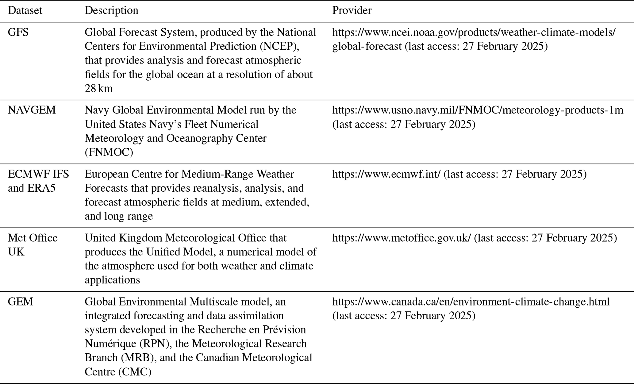
Table 1 Examples of global atmospheric forcing products and providers. Adapted from Alvarez Fanjul et al. (2022).

In addition to the primary classes of flux datasets described above, flux fields for OOFSs are available from several other types of products. An example is surface fluxes available from various ocean synthesis efforts; that is, ocean models with data assimilation such as the Estimating the Circulation and Climate of the Ocean (ECCO) model (Stammer et al., 2004). These systems are typically forced by global atmospheric reanalysis fields which are then adjusted as a result of the assimilation and optimization process. Similarly to atmospheric reanalyses, air–sea datasets based on delayed-mode synthesis efforts are suitable for testing OOFSs during their development stages.

3 Implementation of atmospheric forcing fields in OOFSs

This section briefly lists methods for implementing ocean–atmosphere fluxes applicable in ocean forecasts, monitoring and reanalyses. The four most common approaches are as follows:

• directly using the atmospheric fluxes produced by NWP systems of national meteorological services. Typically, NWP systems produced by national meteorological services provide atmospheric surface forcing fields to OOFSs in order to compute water, heat, and momentum fluxes. Such fields may also be supplemented by real-time or near-real-time observations, e.g. satellite data, and other averaged datasets including climatology. For example, Trindade et al. (2020) show how scatterometer-derived wind stress can be used to remove NWP model output local biases. Relevant points to consider when using NWP products in OOFSs are data availability, space–time resolution, and domains for regional/coastal OOFSs (see next section). Table 1 provides examples of widely used global atmospheric NWP and reanalysis products.

• using a so-called “bulk” forcing to simulate the near-surface ocean–atmosphere interactions (Josey, 2011). This method permits the use of sea-surface temperature to compute in line and at each time step the turbulent fluxes and upward radiative fluxes and so to introduce a pseudo-coupling. The bulk forcing requires some atmospheric data: air temperature, air humidity, downward shortwave radiation, downward longwave radiation, precipitation, wind speed, and wind stress. The latter can also be calculated from the wind speed. This method raises the same questions as the previous one, plus the choice of the surface flux parameterization and associated choice of coefficients in the bulk formulae.

• using an intermediate simplified atmospheric model (e.g. Lemarié et al., 2021) driven by atmospheric NWP 3D fields and producing ocean–atmosphere fluxes consistent with the ocean evolution and resolution. This method is more complex than the bulk forcing but improves the feedbacks between the upper ocean and lower atmosphere, especially when the intermediate atmospheric model and the ocean model have the same horizontal resolution, in order to provide high-resolution atmospheric fields (Alvarez Fanjul et al., 2022).

• using a fully coupled ocean–atmosphere modelling system where the surface fluxes are an integral part of the coupled system. Although this is the most advanced physical approach to simulate ocean–atmosphere interactions, it comes at a relatively high numerical/computational cost, including the initialization/assimilation. The advantages of a fully coupled system (compared to the first three methods) are that there is no (or, for regional OOFSs, a lower) dependence on the data availability from external sources and that it ensures a two-way consistency of the ocean–atmosphere fluxes.

4 Applications of air–sea flux datasets in OOFSs

Each of the implementations described above has its own advantages and disadvantages, and it is not possible to recommend a best air–sea flux product based on the method for implementing surface fluxes in an ocean model; rather, the choice of flux dataset must be guided by the scientific feasibility and by the application in mind. For example, near-real-time NWP products are needed for operational ocean forecasting purposes, whereas a reanalysis product might be appropriate and more convenient to use during the development stages of an OOFS and for validation purposes. Hence, we offer some examples of possible air–sea forcing fields in OOFSs in Table 1, but they are by no means complete or prescriptive.

4.1 Applications in global OOFSs

Global NWP models, like those operated by centres listed in Table 1 at present, have typical horizontal grid resolutions of 20 km or better (and 60 vertical levels or more). With this kind of horizontal resolution, it is possible to capture large-scale synoptic weather phenomena and associated signals in the air–sea fluxes used to force ocean models.

However, in NWP systems with such grid resolutions, it is not possible to accurately simulate smaller-scale ocean–atmosphere interactions, such as oceanic fronts and orographic features like land–sea circulation or air–sea interactions associated with mesoscale oceanic eddies, noting that the synoptic (eddy) scale in the ocean is on the order of ∼ 100 km, which is about 1 order of magnitude smaller than in the atmosphere at about ∼ 1000 km.

Atmospheric forcing fields are typically interpolated onto the respective grid points of the ocean model, e.g. momentum fluxes onto the velocity grid points, air–sea heat fluxes onto the temperature grid points and evaporation minus precipitation onto the salinity grid points of the ocean model (plus volume or mass flux in the continuity equation). This interpolation can be accomplished either by using an internal interpolation routine of the ocean model; by using bulk formulae at the ocean grid to calculate surface fluxes of heat, freshwater, and momentum; or by using specific coupling software, e.g. Craig et al. (2017), for fully coupled ocean–atmosphere–wave–sea–ice models.

4.2 Applications in regional and coastal OOFSs

There is a plethora of regional and coastal ocean models with fixed, variable, and adaptive grids and with horizontal resolutions often in the 10–100 m range (Kourafalou et al., 2015). It is therefore not possible to provide specific guidance about the appropriate choice of air–sea fluxes required for these types of models.

Regional- to basin-scale OOFSs are typically forced with air–sea fluxes from the latest high-resolution global NWP systems, e.g. O'Dea et al. (2012). In contrast, coastal OOFSs require a different approach. Coastal air–sea circulation and topographic features, like small islands and their interactions with air–sea fluxes, are not reproduced by global-scale atmospheric models; hence, much higher resolution coastal atmospheric models are needed to provide reliable upper-ocean boundary conditions. This can be accomplished by direct coupling of high-resolution atmospheric models to coastal ocean models or by using air–sea fluxes from a stand-alone NWP higher-resolution coastal model (Hordoir et al., 2019). Other examples of regional atmospheric models are the UK Met Office Unified Model–JULES Regional Atmosphere and Land configuration (Bush et al., 2023) and the Weather Research and Forecasting (WRF) model (Skamarock et al., 2008). Either way, these atmospheric models need to be nested (in multiple) within coarser-resolution regional and/or global models which provide lateral and upper boundary conditions. This is an active field of R&D, where the development of coastal NWP and OOFSs often goes hand in hand with efforts to develop fully coupled ocean–atmosphere forecasting systems. However, it should be noted that, for both components, atmosphere and ocean, not just suitable lateral boundary conditions from coarser-component models are required, but it is also highly desirable to have an appropriately dense atmospheric and oceanic observing system to constrain these models and improve (coupled) forecasts.

High-resolution air–sea fluxes, which are based on remotely sensed fluxes, can also be used to evaluate the quality of the forcing fields in coastal ocean models. An example is the synthetic aperture radar (SAR)-based remotely sensed regional ocean wind speed and direction database, which has been made available by the Australian Integrated Marine Observing System (Khan et al., 2023). The dataset is a kilometre-resolution ocean wind speed and direction database over coastal seas of Australia, New Zealand, the western Pacific Islands, and the Maritime Continent. It is obtained from Europe's Copernicus Sentinel-1A and Sentinel-1B SAR satellites from 2017 up to the present. The dataset is a first of its kind in the region and captures the spatial variability in coastal ocean winds over a wide swath (250 km). However, and, as stated above, any SAR-derived wind stress product available to date and its use for OOFS development purposes needs to be treated with caution and should be assessed on a case-by-case basis.

5 Conclusions

This study provides some information about the diverse range of air–sea flux datasets that are now available for the community to use as air–sea forcing in OOFSs. NWP systems provide the majority of flux products to force today's OOFSs. Generally speaking, the quality and usefulness of these datasets are influenced by the spatial and temporal resolutions of remotely sensed and in situ observations that are assimilated into the NWP systems and are limited by associated biases which should be taken into account when choosing such datasets. Consequently, air–sea flux datasets for OOFSs should be chosen with the applications and users of the outputs in mind.