the Creative Commons Attribution 4.0 License.
the Creative Commons Attribution 4.0 License.
 | 30 Sep 2024 | OSR8 | Chapter 3.1
Oceanographic preconditions for planning seawater heat pumps in the Baltic Sea – an example from the Tallinn Bay, Gulf of Finland
Ilja Maljutenko
Priidik Lagemaa
Rivo Uiboupin
Urmas Raudsepp
The use of low-temperature seawater heat for renewable energy installations is demonstrated with an example from the Tallinn Bay, Baltic Sea, based on Copernicus Marine Service reanalysis data. Tallinn and its surrounding seaside counties are home to about half a million people and produce about half of Estonia's gross domestic product (GDP). The Tallinn Bay with an area of 223 km2 extends to the north and has an open connection to the Gulf of Finland. Depths more than 50 m that cover the halocline already appear at a distance of 3–4 km from the coast. Surface layers get too cold during winter to be used in heat pumps for district heating; therefore, a feasible option is to pump slightly warmer seawater from the deeper halocline layers. The lowest monthly mean halocline temperature – down to 2.6 °C at 50 m depth and 3.3 °C at 70 m – is found in March and April based on reanalysis data from 1993–2019. The seawater seasonally cools below 3 °C on average on 1 January at 20 m depth and on 12 February at 50 m depth. At the 70 m depth, the average start of T<3 °C was calculated on 28 February, although only 14 winters out of 26 had such water present; in 12 winters the condition T>3 °C was always fulfilled. The median number of cold days is 11, with a maximum of 128 d in the winter 1993/1994 when stratification became rather weak due to the prolonged absence of Major Baltic Inflows of saltier and warmer North Sea waters. During the recent warmer period of 2009–2019, the start of the cold seawater period was delayed on average by 5–10 d. Tallinn has, among other Baltic Sea cities and industrial sites, a favorable location for seawater heat extraction because of the short distance to the unfreezing sub-halocline layers. Still, episodically there are colder-water events with T<3 °C, when seawater heat extraction has to be complemented by other sources of heating energy.
- Article
(5547 KB) - Full-text XML
- BibTeX
- EndNote


Table 1Copernicus Marine Service and non-Copernicus products used in this study, including information on data documentation.
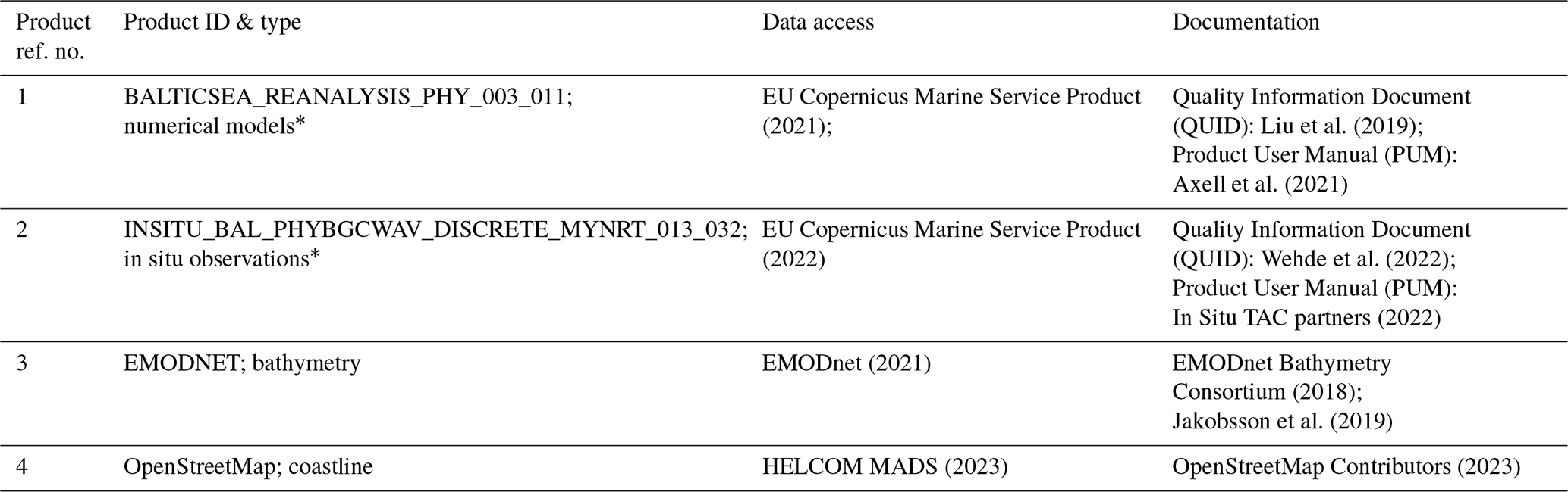
* Data set updated during publication (see the “Disclaimer” section).
New developments in district heating (e.g., Lund et al., 2018) focus on the gradual exclusion of fossil fuels and transfer to 100 % renewable energy sources. Among the latter, large-scale heat pumps are considered to be an important component of the new energy systems. One energy source for the heat pumps is seawater (Bach et al., 2016) that has a stable temperature during the winter compared to the air temperature. Seawater heat pumps take seawater from the locations of appropriate temperature into the shore unit that transforms its low temperature to higher temperature suitable for district heating. Regarding feasibility studies, Su et al. (2020) performed a spatial evaluation of seawater-source heat pump performance along the coast of China depending on technical options and the thermal regime of seawater or other heat sources (wastewater, groundwater etc.). Pieper et al. (2019) evaluated combinations of heat pumps based on data from Copenhagen and noted that in shallow-water conditions seawater heat may contribute 14 % of the total heating energy. An important issue in coastal waters of ice-prone seas is to avoid lowering of temperature in the heat pump system below the freezing temperature, which depends on the salinity. Water temperature during winter usually increases at depth, and hence, even depths of a few tens of meters may be sufficient to avoid freezing temperature. One of the world's largest seawater heat pumps, built in Ropsten in Stockholm and operational since 1986, was designed to work with the lower limit of input water temperature of +2.5 °C (Friotherm, 2017). The system pumps large-volume flows of water from the 15 m depth; by cooling the water down to +0.5 °C, the system yields in total 180 MW from six units. In the Danish town of Esbjerg, a 60 MW seawater heat pump is in the construction phase to replace the town's existing coal power plant for heating purposes (CleanTechnica, 2023). The study by Volkova et al. (2022b), summarizing geographical and economic factors, concluded that among the Baltic countries, seawater is the best natural heat source in Estonia, but river water has higher potential for the other two countries. Contemporary housing also needs district cooling during the summer that can be performed based on the seawater (Volkova et al., 2022a).
Tallinn is a seaside city with about half a million inhabitants on the coast of the Gulf of Finland, Baltic Sea, where the use of seawater heat for district heating is currently under consideration. Unfortunately, during the winter period, i.e., when the highest demand for heating housing exists, coastal seawater at shallow depths may cool down close to the freezing temperature, which may hamper the efficiency of using the heat pumps. It is known from the larger Gulf of Finland area that during summer the mean halocline depth is located at about 67 m, keeping the temperatures in the range of 2.2–5.0 °C depending on the transport of deep, more saline waters from the open Baltic Sea (Liblik and Lips, 2011). The waters in the halocline and below are rather isolated from direct vertical heating and cooling; therefore, their temperature is more stable than in the surface layers. As a systematic analysis of the near-bottom water temperature in the Tallinn Bay is missing, the present study focused on the exploration of the new public data sets made available by the EU Copernicus program. The Copernicus Marine Service (https://marine.copernicus.eu/, last access: 13 February 2021) provided regular Baltic Sea reanalysis data during 1993–2019 with about a 3.7 km grid step, combining both modeling and observations (Table 1, product ref. no. 1).
The aim of the present study is to determine the basic features of seawater temperature variability, necessary for the evaluation of the feasibility and efficiency of using seawater thermal energy for heating and/or cooling of a city's built environment. The presentation of data and methods is followed by providing results and discussion with a focus on subsurface temperature variations with respect to the cold-water periods. The paper ends with recommendations for further studies and conclusions.
2.1 State of knowledge on oceanographic conditions in the Baltic Sea
The Baltic Sea is a multi-basin semi-enclosed sea (Fig. 1a) filled with brackish waters. Its temperature regime (Leppäranta and Myrberg, 2009) is to a great extent forced by the seasonal cycle of atmospheric heat fluxes that extend down to the thermocline during summer and to the halocline during winter (Fig. 1b). In halocline and deeper layers, temperature is determined mainly by the deep-water transport of the waters originating from the North Sea (Leppäranta and Myrberg, 2009). However, these waters are significantly transformed on their pathway from the Danish straits through the Baltic Proper to the Gulf of Finland.
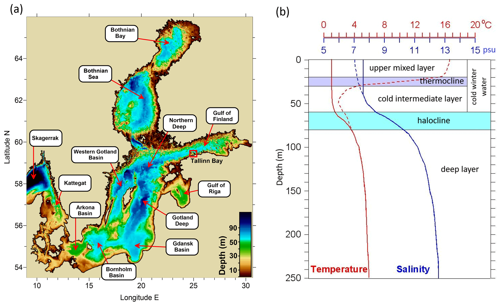
Figure 1Topography and basins of the Baltic Sea (a). The Baltic Proper includes Arkona Basin, Bornholm Basin, Gdansk Basin, Gotland Deep, and the western Gotland Basin. Typical vertical stratification in the Gotland Deep (b, adopted from Elken and Matthäus, 2008) in summer (dashed lines) and winter (solid). The location of Tallinn Bay is shown in (a) with a red box.
While temperature and sea ice respond rapidly to changes in atmospheric heat fluxes, variations in salinity are governed mainly by lateral transport processes, resulting together with diapycnal mixing (i.e., mixing across the surfaces of constant water density) in response times of many decades (e.g., Omstedt and Hansson, 2006; Elken et al., 2015). The Gulf of Finland is an elongated sub-basin of the Baltic Sea, which has many specific features (Alenius et al., 1998). Stratification is generally composed of the following layers.
Upper mixed layer. Generally, the upper mixed layer is vertically rather uniform due to high mixing rates generated by winds, waves, and convection during cooling (Leppäranta and Myrberg, 2009). During summer, it typically has a thickness of 20 m in the Gulf of Finland (Liblik and Lips, 2011). On calm and sunny days, a thin warm “skin” layer may occur just at the surface. However, with increasing wind speed the whole upper layer undergoes overall mixing again. The yearly temperature maximum occurs in July or August depending on the region and yearly atmospheric conditions (Haapala and Alenius, 1994). During the autumn cooling period, the upper layers become hydrostatically unstable. If cooled water with higher density appears on top of warmer and less dense water, then instability generates convective mixing (Maljutenko and Raudsepp, 2019). As a result, mixed layer temperature decreases but its thickness increases until its lower boundary has eroded down to the halocline or to the bottom, whichever is shallower. Shallow sea areas warm and cool faster during spring and autumn (also called differential heating), respectively, because of the smaller water mass of the water column compared to deeper ocean areas.
Cooling of the upper layer is limited during winter by the salinity-dependent freezing point of seawater. For salinity values of 5, 6, and 7 psu, the freezing point is −0.27, −0.33, and −0.38 °C, respectively. The salinity-dependent temperature of maximum density Tmax influences upper-layer dynamics during the cold period as well. For fresh water, Tmax=4 °C, and for typical Baltic surface salinity of 7 psu Tmax is about 2.5 °C.
Thermocline. During summer, a sharp temperature drop at depth develops below the upper mixed layer. Individual instant profiles may exhibit the sharpest thermoclines with temperature drops from 5 to 10 °C per 5 m (Fig. 1b), and the mean summer thermocline thickness in the Gulf of Finland is 14 m (Liblik and Lips, 2011). With respect to the mean seasonal cycle, the thermocline may perform up- and downward motions with periods from a couple of hours to several days. Vertical movement of the thermocline of 10 m or even more creates significant near-bottom temperature variations. A special dynamical feature of the thermocline is upwelling, when cold waters (sometimes below 5 °C) may be found at the surface of coastal areas during summer (Aavaste et al., 2021). In the Gulf of Finland, upwelling occurs near the Estonian coast during easterly winds and near the Finnish coast during westerly winds (Uiboupin and Laanemets, 2009).
Cold intermediate layer. Cold waters from the last winter remain below the thermocline, trapped through the whole summer, until autumn cooling pushes the thermocline significantly downwards. In the Gulf of Finland, lowest summer temperature (from 1.3 to 3.6 °C) has been found on average at 42 m depth (Liblik and Lips, 2011).
Halocline and deep layers. This layer is formed by lateral (horizontal) transport of saline waters originating from the North Sea. Regular saline water inflow is complemented by the events of Major Baltic Inflows (MBIs) of large volume and high salinity; they occur sporadically with intervals from years to decades (Raudsepp et al., 2018). Depending on the seasonal timing of the MBI, there may be pulses of warmer or colder water reaching the deep areas of the Baltic Proper (Elken et al., 2015). For example, in the Gotland Deep at the 175 m depth, temperature varied during 1997–2013 between 4.5 and 7.0 °C depending on the type of the MBI. When large volumes of new water arrive to the Gotland Deep, the old water is pushed to the deep layers of the Gulf of Finland. After the 2014 December MBI, the first effects occurred in the Gulf of Finland in 9 months, whereas the arrival of the former northern Baltic Proper deep-layer water was observed (Liblik et al., 2018). Deep-layer temperature dynamics in the Gulf of Finland are also affected by the wind-dependent estuarine circulation reversals that may drastically reduce the stratification for several weeks (Elken et al., 2003).
Tallinn Bay is deep enough to have all of the above-described water column layers present. Its short-term hydrographic variability is characteristic of the southern coast of the Gulf of Finland: upwelling occurs during the persistent westerly and southwesterly winds, and pulses of more saline and less saline water observed in the southern Gulf of Finland also appear in the bay.
From May to July, the seasonal cycle of temperature in the central part of the Gulf of Finland shows delayed temperature increase of the layers 20–40 m during the warming season (Haapala and Alenius, 1994). The seasonal upper-layer temperature maximum usually develops in August. In the course of the cooling period, the thermocline deepens to 30 m (i.e., temperature of that level becomes equal to surface temperature) in September and 40 m in October. The 50 m depth level lies in the cold intermediate layer at temperatures below 8 °C through the year. Average temperature in the halocline (60–90 m) is stable, ranging from about 3 °C in February and March to 5 °C in November and December.
Sea surface temperature can be acquired in detail using regular satellite images, but subsurface data can be observed only using sparse in situ techniques. Elken et al. (2015) summarized that during 1990–2008, sea surface temperature increased in the Gulf of Finland at a mean rate of 0.8 °C per decade. Liblik and Lips (2019) explored large numbers of observations conducted in the water column. They have shown that from 1982 to 2016 the temperature of the Gulf of Finland was increasing on average at a rate of about 0.5 °C per decade, whereas faster warming has been detected in the thermocline (20 m) and at deeper (70 and 80 m) depth levels. Re-inspection of temperature observations in the Gulf of Finland from the HELCOM/ICES database at the 70 m depth level reveals that average deep-water temperature increased from 3.5 °C in 1988 to 5.2 °C in 2020. Oceanographic regional climate projections until 2100 have projected an annual increase in temperature in the Gulf of Finland of 0.2–0.4 °C per decade (Meier et al., 2022).
2.2 Data
2.2.1 Copernicus Marine Service reanalysis data for the Baltic Sea
We use the Baltic Sea physical reanalysis product (Axell, 2021) prepared within the Copernicus Marine Service (product ref. no. 1). This reanalysis covers the whole Baltic Sea with adjacent North Sea areas, presenting data on sea level, ice, water temperature, salinity, and currents. It has about a 3.7 km grid step and is the most advanced combination of numerical modeling made using the NEMO model and observations. The data set consists of daily mean reanalysis data from 1 January 1993 to 31 December 2019. The gridded data have a maximum of 56 vertical levels down to 361 m. Layer thickness is about 3 m in the upper levels but increases to about 6.3 m in the deepest point of the Tallinn Bay area, which has altogether 21 depth levels.
The quality of the reanalysis product was vigorously checked against observational data by Liu et al. (2019). The report concluded that the mean bias of water temperature was less than 0.1 °C and the remaining root mean square deviation (RMSD) was less than about 0.7 °C. Comparing with individual independent observations that were not included into the reanalysis procedure, the RMSD is generally between 0.4 and 1 °C. The largest RMSD values above 1.4 °C were found in the Kattegat and the Gulf of Finland. In the Tallinn Bay, the reanalysis results are compared to the independent sea surface temperature observations in Sect. 2.3.
The grid cells of the NEMO model are shown in Fig. 2, overlaid on the coastline and topography map of the Tallinn Bay. Although depths 40–70 m are evident in the inner bay, the reanalysis grid cells of the Baltic-wide product are too coarse to resolve the details of the coastline and topography. Setting up a more detailed topography for oceanographic reanalysis, dedicated to Estonian marine areas, is in the implementation phase.
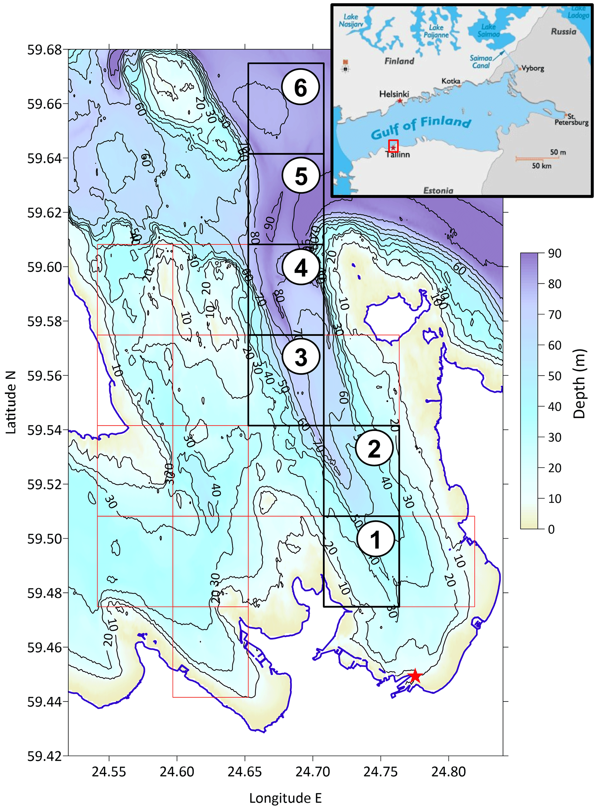
Figure 2Map of the Tallinn Bay area with grid cells of the Copernicus Marine reanalysis data (product ref. no. 1) shown as boxes. The location of the Tallinn Bay is shown on the map of the Gulf of Finland, inset in the upper-right corner. The analysis uses data from bold cells noted by numbers. The red star denotes the location of the coastal automatic observing station. Depth data on the arcmin (ca. 58 and 116 m along longitude and latitude) grid were adopted from EMODNET bathymetry (product ref. no. 3). The coastline has been adopted from the compilation by HELCOM (product ref. no. 4).
For the present analysis, data from six grid cells were selected. The data on the original grid were converted to 10 m depth intervals.
2.2.2 Observations
Regular temperature observations are available from the automatic coastal station (59.449351° N, 24.775448° E) located in Tallinn Harbor (Fig. 2) from 1 January 2008 to 14 April 2018 (product ref. no. 2). The sea level part of the observing station has been described by Lagemaa et al. (2011). The raw data have been recorded mostly with a 5 min interval. After elimination of sensor and communication errors, a set of daily mean temperatures was generated to compare with reanalysis data. The same data, processed to the 1 h interval, are available from the Copernicus Marine Service.
2.3 Comparison of reanalysis data with observations
While observational data record the “point” values of sea surface temperature with a 5 min interval and are usually averaged to hourly values, the reanalysis data set presents the average temperature over ca. 3.7 km size grid cells as daily mean values. It means that reanalysis data do not present small-scale and short-term local temperature variations near the observation point. Still, it is interesting to compare how well point observations match averaged reanalysis data. Point observations reveal a number of short-term anomalies from the regular seasonal course (Fig. 3). Their origins are in (1) calm weather local anomalies, when a warm skin layer develops, mostly during spring; (2) faster heating and cooling in shallow coastal sites; and (3) cold waters due to wind-induced upwelling. In all the cases, the spatial and temporal scales could be too small to be captured by the coarser reanalysis data. This study did not focus on a detailed analysis of “negative temperature anomaly” events, but we can conclude that in many cases the observed events are also evident in the reanalysis data. Since the upwelling areas cover up to tens of kilometers and may exist for several days or a week (Uiboupin and Laanemets, 2009), these events are captured well by the reanalysis data.
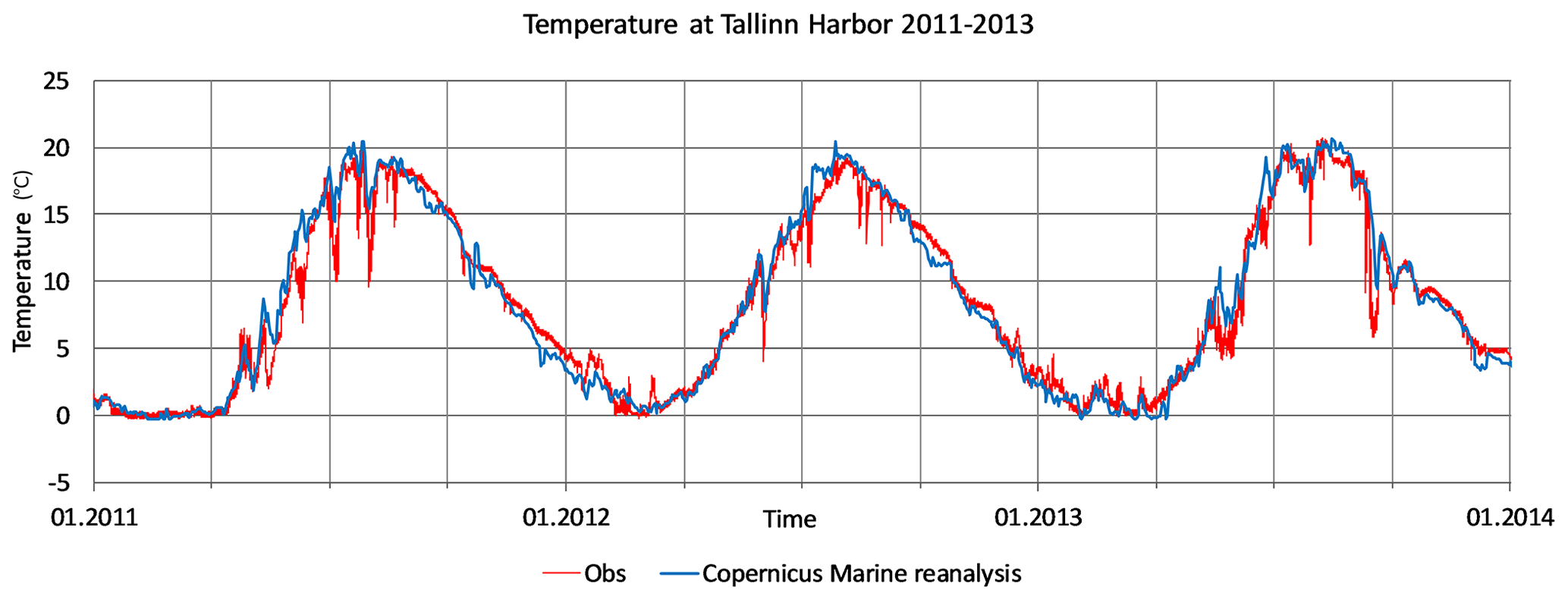
Figure 3Example of near-surface temperature time series in 2011–2013. Shown are the automatic observations at Tallinn Harbor with a 5 min interval averaged to hourly values (red) (product ref. no. 2) and daily Copernicus Marine reanalysis data at point 1 (blue) (product ref. no. 1). For locations, see Fig. 2.
Statistical comparison of surface reanalysis data with daily mean observations over existing data pairs reveals their good match. Bias is −0.12 °C and RMSD (root mean square difference) is 1.3 °C. Both time series contain a strong seasonal signal, with its variance exceeding 90 % of the total variance. While the original time series are highly correlated with the Pearson coefficient of determination at R2=0.96, removing the mean seasonal cycle from both of the time series reduces the correlation to R2=0.44. A histogram of the difference between observations and reanalysis (not shown) shows that on average observations reveal slightly higher temperature (the maximum is shifted by 0.2 °C), but occasionally much smaller observed temperatures occur. Such outliers can neither be explained by the local coastal effects in observations nor resolved by reanalysis.
3.1 Seasonal temperature course and its variations
The temperature of the Tallinn Bay undergoes a similar seasonal cycle as described in Sect. 1. In the offshore area (point 6, Fig. 2) the upper layer is gradually warmed up from April to July (Fig. 4a). During summer, the upper mixed layer has 10–20 m thickness, whereas the annual temperature maximum, determined from the original non-averaged data, varies between 16 and 23 °C. In August, the maximum vertical gradient in the thermocline is found at about 25 m depth. During autumn, the upper layer and the thermocline are eroded down to 40 m where inherent salinity stratification (Fig. 4b) blocks further erosion. During winter, the upper layer may be cooled to the freezing point, which is from −0.27 to −0.33 °C for salinities from 5 to 6 psu. Below the thermocline, monthly mean temperature ranges from 2.4 to 7.4 °C at 40 m depth and from 3.4 to 5.2 °C at 70 m depth (Fig. 4a). Deeper temperature variations below 40 m are influenced by the seasonal dynamics of the halocline: intensified transport of more saline (and warmer) waters from the open Baltic occurs below 50 m in late spring and summer (Fig. 4b). The highest temperature occurs in deeper layers in November and December as a delayed response to the summer heating at the surface; the lowest temperature values are found on average in March and April when the weakest vertical gradients in the halocline occur.
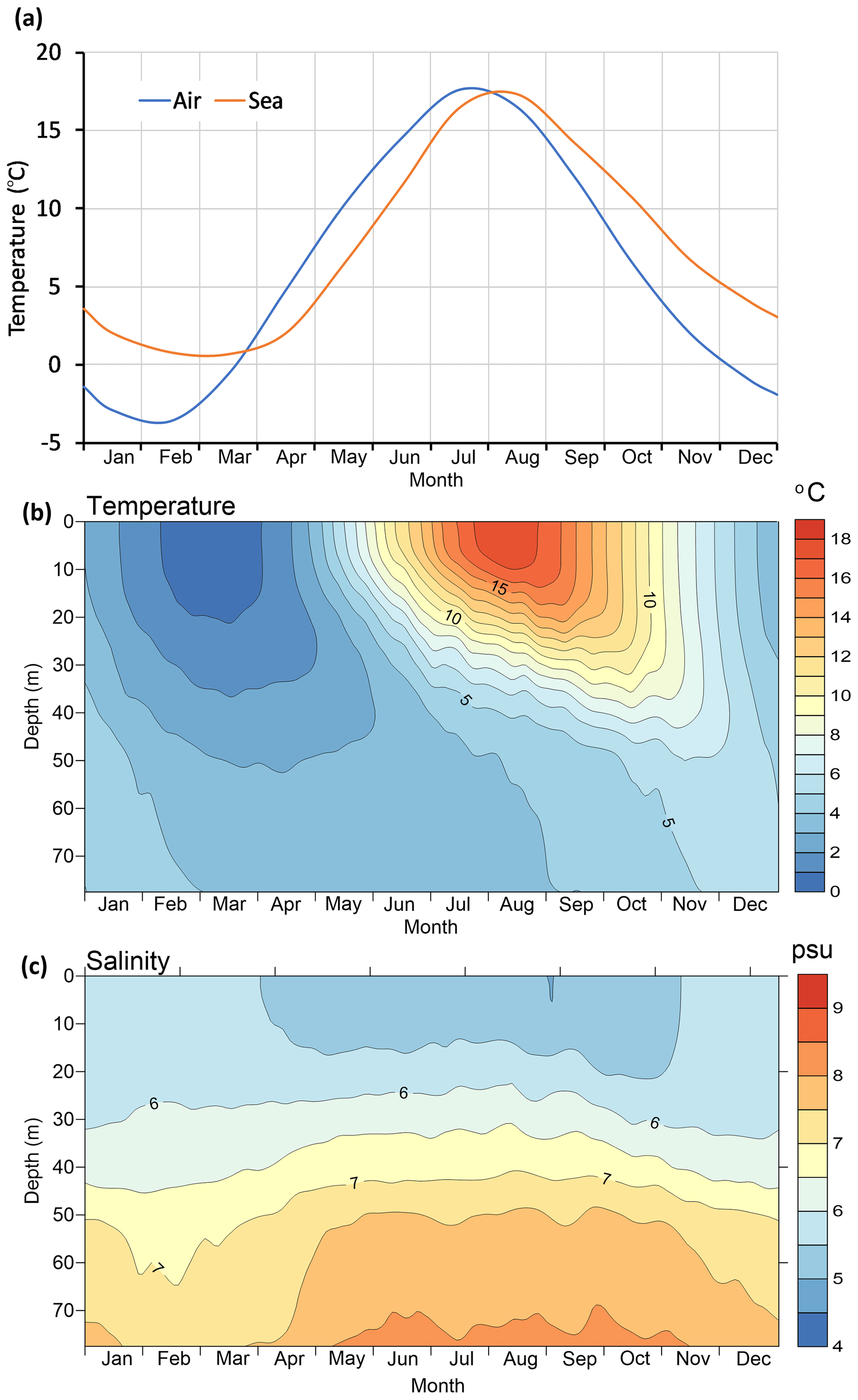
Figure 4Monthly mean air temperature and surface water temperature in the Tallinn Bay (a) and mean seasonal depth distribution of temperature (b) and salinity (c) in the Tallinn Bay at reanalysis point 6 (Fig. 2) as a function of time of the year (month) and depth. Data are from Copernicus Marine reanalysis for 1993–2019 (product ref. no. 1).
Although in the six selected reanalysis points (their locations are in Fig. 2) the mean seasonal temperature curves are rather similar (Fig. 5), the spread of the actual data is rather high. Histograms of weekly mean temperature reveal during the summer months a range from 4.5 to 22.5 °C at the depth of 10 m, with a maximum in overall seasonal mean of 16 °C. The cold anomalies are rather rare – summer temperatures below 10 °C cover only 7 % of occurrence frequency. During winter months, temperature variability is confined between −0.2 and 3.5 °C at 10 m depth, while at 50 m the limits are 0.5 and 5.4 °C. Mean seasonal data from individual reanalysis points reveal minor horizontal variations between the points compared to their temporal variations. For example, during the winter when deep seawater is needed for the heat pump, the pointwise monthly mean temperature varies at 50 m depth between 2.6 and 2.8 °C in March, but it has a mean seasonal maximum of about 5.9 °C in November and December. Detailed analysis reveals that the temperature of deep layers below 40 m depth can be considered practically uniform over the bay area on scales of a few kilometers and a few days, which is sufficient for the baseline evaluations of oceanographic conditions for seawater heat pumps.
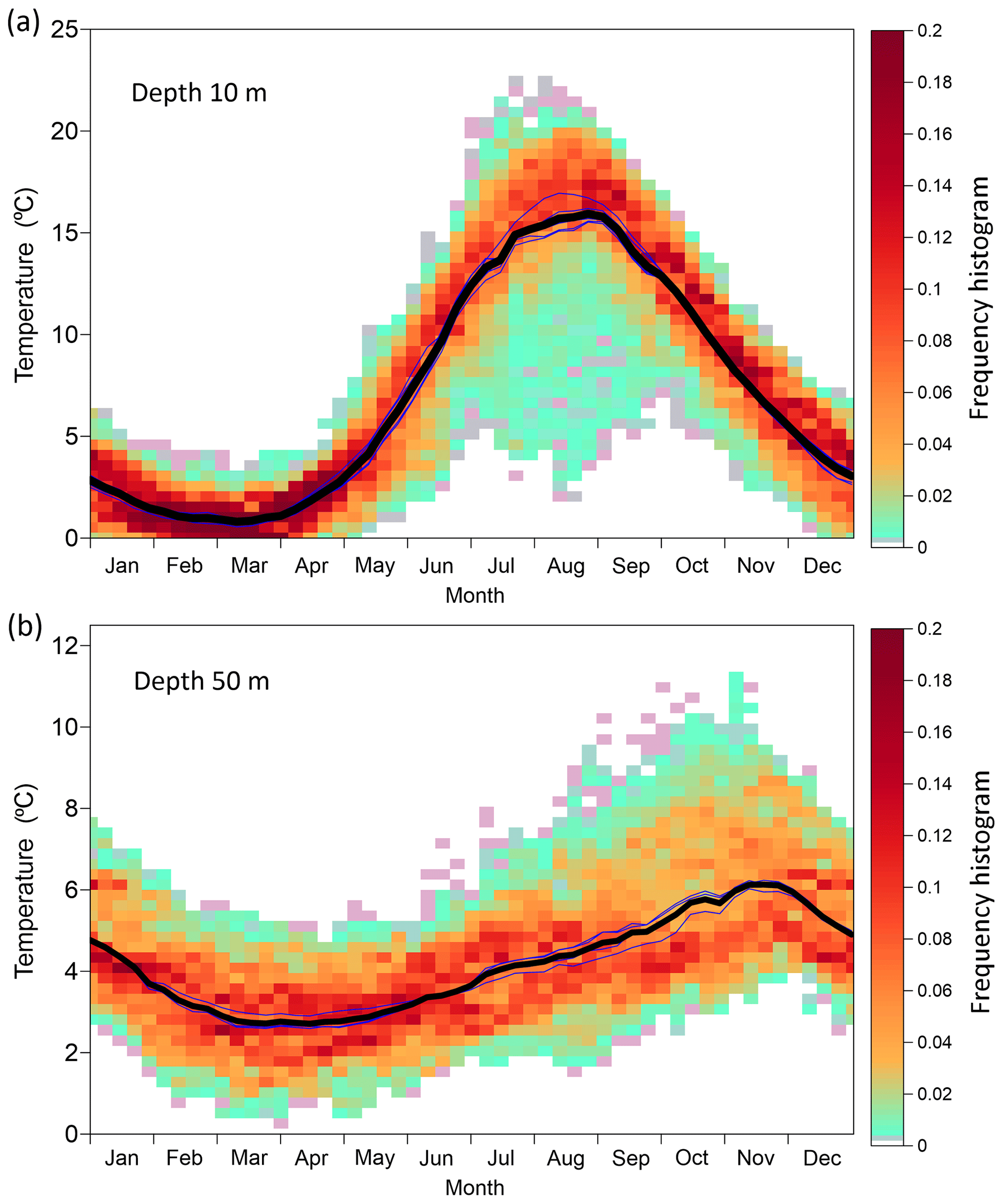
Figure 5Mean seasonal curve (black solid line) and seasonal temperature histogram (color image) in Tallinn Bay at depths 10 m (a) and 50 m (b). Shown are also mean temperature curves for individual horizontal points (thin lines). Copernicus Marine reanalysis data from 1993–2019 (product ref. no. 1) taken from six locations (Fig. 2) are processed with 7 d (weekly) intervals. The temperature histogram bins are 0.5 °C for 10 m depth (a) and 0.25 °C for 50 m depth (b). For each week, the sum of histogram frequency shown by the color scale is 1.
3.2 Statistics of extractable seawater heat
The data were segmented into 26 yearly heating-centered periods from 1 July to 30 June. For the data visualization of each year, a date–year column diagram was drawn, where the color stripes in the column correspond to the actual temperature in a specific year based on the defined color scale (Fig. 6). Results show that at both the 50 and 70 m level of the offshore point 6, the highest temperatures above 4.0 °C occurred every year, but the duration and timing are variable. During the winters 2000–2001, 2007–2008, and 2008–2009, deep layers were warmer than usual through the whole year. In several years, the warmer deep waters were dominant until February or March. There were also years when colder waters were present in summer and extended to autumn, a time when deep-water temperature started to increase.
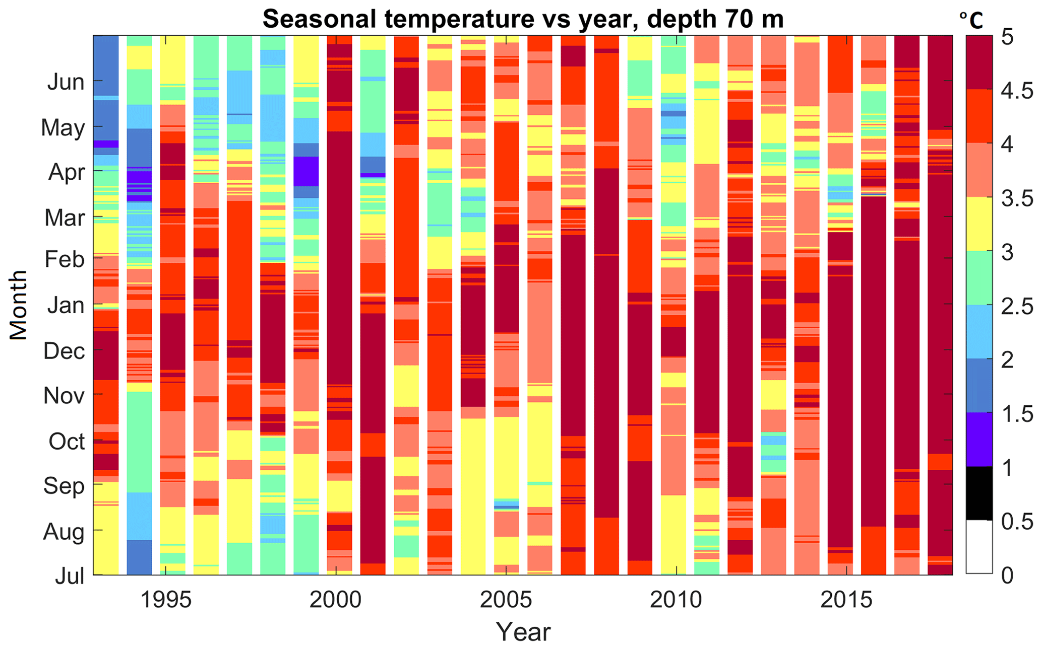
Figure 6Temperature diagrams in Tallinn Bay at 70 m depth as a function of year (horizontal axis) and calendar day (vertical axis), calculated from Copernicus Marine reanalysis data (product ref. no. 1).
We define seawater heat as extractable when water temperature exceeds some predefined value, while cold water occurs when the temperature is below that limit. Cold period durations and start dates were determined by evaluating running 9 d slices of temperature criteria fulfillment in the time series. Shorter-duration spikes with fewer than four fulfillments were considered not fulfilled. For the heat pump problem, the time series were limited to periods from 1 October to 30 April, which is usually the heating period of city districts. The results reveal that at a depth level of 20 m (not shown), the water was cold in every winter. Even in the mildest winter of 2007/2008, water with T<2 °C was present for several days. Going further to the deeper layers of 50, 60, and 70 m, the limit T<2 °C is normally not found (except for very cold winters in 1993/1994, 1994/1995, 1999/2000, and 2010/2011), and even cases with T<3 °C were rather rare.
Profiles of the mean number of non-cold days (when heat extraction is considered possible) reveal that favorable periods corresponding to different temperature limits are minimal in the surface layer down to 20 m (Fig. 7). Further, with increasing depths, extractable seawater heat becomes more frequent. A significant increase in the duration of seawater-based heating occurs from 30 to 50 m depth, from 107 to 166 d for 3 °C, and from 149 to 200 d for 2 °C. Considering the recent period 2009–2019, selected to cover the positive temperature trend, the mean duration of non-cold days was generally 5–10 d longer than for the whole period of 1993–2019, whereas the largest increase of up to 20 d was found in the deepest layers at 60 and 70 m.
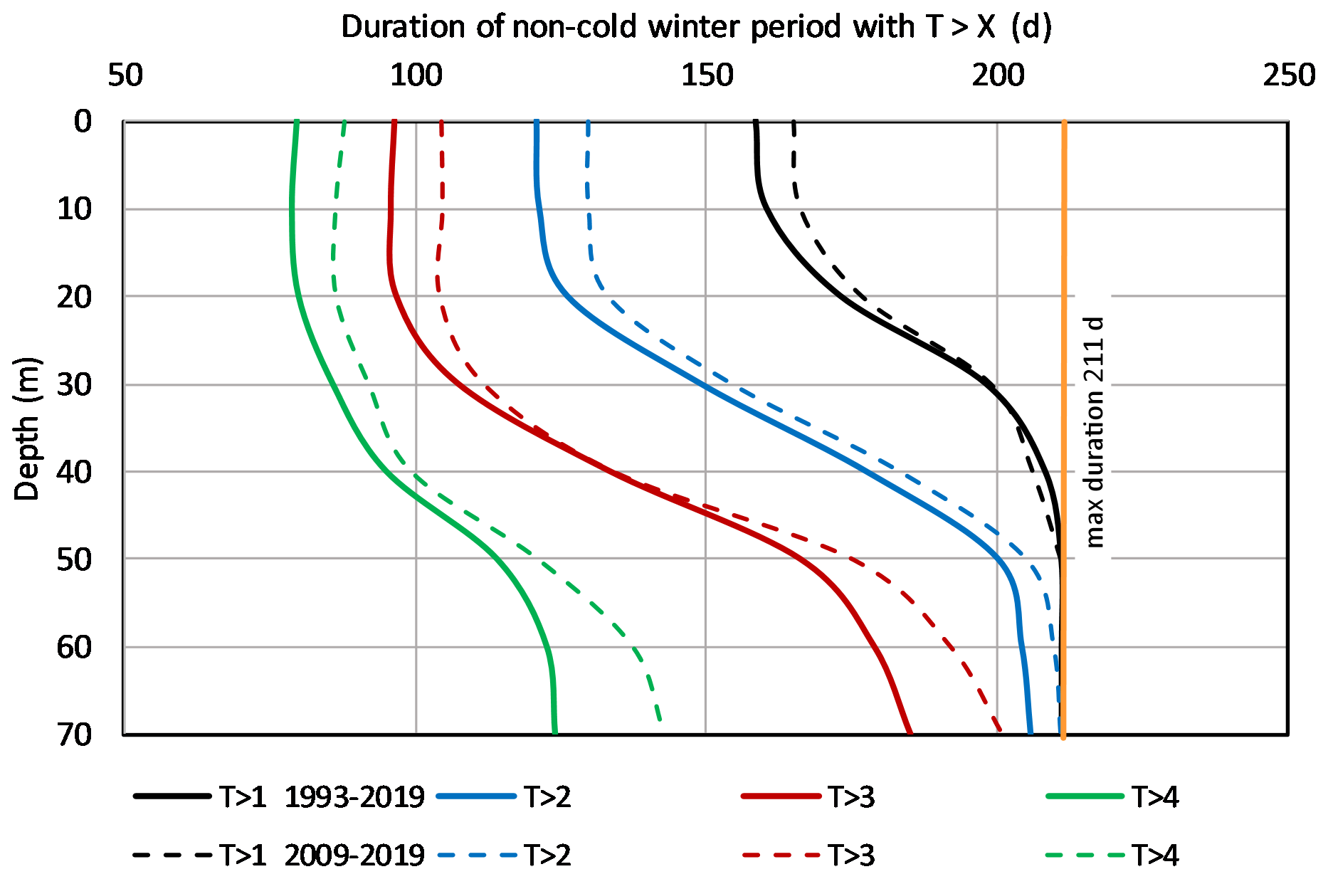
Figure 7Profiles of the mean number of non-cold days for the reanalysis point 6 (Fig. 2). X=1, 2, 3, and 4 °C as shown in the legend. Copernicus Marine reanalysis data are from 1993–2019 for the full period (solid line) and for the recent 11 years (2009–2019; dashed line). Data are taken from 1 October to 30 April (211 d) of each year (product ref. no. 1).
Profiles of mean start dates of cold periods, when additional heating must be switched on, were calculated from 1 November of each year (Fig. 8). In both offshore and coastal waters the start dates are nearly the same. The temperature goes below a certain limit first at the surface layer and later in the deeper layers. Seawater temperature becomes less than 3 °C on average on 1 January at 20 m depth and on 12 February at 50 m depth. At the 70 m depth, the average start of T<3 °C was calculated on 28 February, although only 14 winters out of 26 had such water present; in 12 winters the condition T>3 °C was always fulfilled. We note that calculations made with the mean seasonal cycle (Fig. 4) always revealed T>3 °C. During the recent warmer period of 2009–2019, the start was delayed on average by 5–10 d. However, this estimation is rather uncertain, since there have been several winters where the criteria T<1 °C, T<2 °C, and T<3 °C have not been met due to dominating warmer waters. Among the winters in 1993–2019, temperature at 50 m depth was above 3 °C for more than 5 d during 9 winters (35 %) and above 2 °C during 18 winters (70 %). The coldest winters, as shown in Fig. 6, with low deep-water temperature were 1993/1994, 1994/1995, 1999/2000, and 2010/2011.
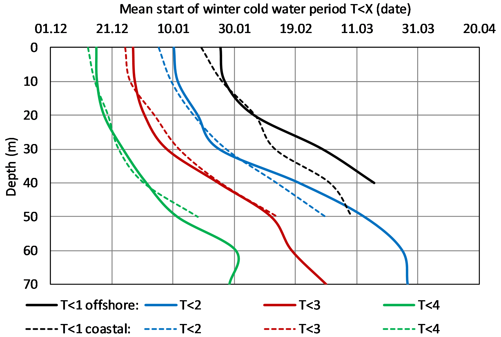
Figure 8Profiles of the mean start date of the cold seawater period. X=1, 2, 3, and 4 °C as shown in the legend. Copernicus Marine reanalysis data (product ref. no. 1) are shown for 1993–2019 from 1 October to 30 April at offshore point 6 (solid line) and internal bay point 3 (dashed line). The locations of points are given in Fig. 2.
The results in Fig. 8 show that statistical properties of cold or warm water occurrence are in the first approach horizontally uniform; i.e., average data from one location can be extended over the entire bay area. Since seawater intake for the heat pump systems is usually located on the bottom, in the small bay its baseline temperature regime can be characterized from the temperature time series of nearby deeper locations.
3.3 Frequency of extractable seawater heat occurrence over the Baltic Sea bottom
Seawater heat pumps can use water with temperature above a certain limit: here T>3.5 °C for non-cold water. Since intake tubes are located on the bottom, “good” locations for seawater heat pump installations are those where non-cold bottom waters of Tbot>3.5 °C occur most frequently, leaving a minimum number of days when an additional (usually less effective) energy source is needed.
Copernicus Marine reanalysis data were used to calculate Baltic-wide non-cold water occurrence frequency on the bottom using the data from the heating period (from October to April) during 1993–2021 (Fig. 9). At each grid cell of the reanalysis data, the near-bottom temperature value for each day was compared to the non-cold criteria, and the counted number of non-cold days was divided by the full number of days during the period, resulting in F=100 % for the regions where Tbot is always >3.5 °C. We may infer that seawater heat is extractable in the regions with F>85 %, as shown by the color scale in Fig. 9. Note that extractable seawater heat is found in the deeper basins of the Baltic Proper, where a permanent halocline exists (Fig. 1).
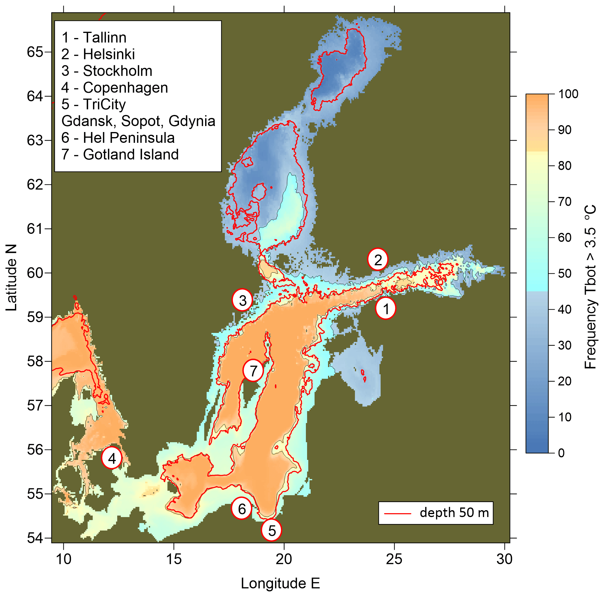
Figure 9Frequency of occurrence of non-cold waters at Tbot>3.5 °C, calculated from the Copernicus Marine reanalysis data for 1993–2021 (product ref. no. 1).
From the socioeconomic viewpoint, favorable locations for seawater heat extraction are a short distance from regions of extractable seawater heat and significant urban and/or industrial areas. Among larger cities, Tallinn has one of the most favorable locations for using seawater heat since the boundary for F>85 % lies just a few kilometers from the coast. In terms of extractable marine heat distance only, the best locations in the Baltic Proper are the western coast of Gotland island in Sweden and the tip of Hel Peninsula near Tri-City in Poland (Gdansk, Sopot, Gdynia), but these regions have only moderate coastal populations. Good locations for seawater heat extractions are found near Copenhagen and other Danish cities, as well as Tri-City in Poland.
The design of seawater heat pumps is a complicated interdisciplinary optimization task (Schibuola et al., 2022). There should be heating or cooling energy users at a reasonable distance from the coast, since a fraction of gained energy is lost to the pumping. In ice-prone (boreal) seas, there should be locations near large-scale users where seawater temperature by depth does not frequently fall below +3 °C. In most cases, it is useful to combine seawater heat energy with other renewable sources, such as groundwater, wastewater, lakes, rivers, and air (Pieper et al., 2022; Volkova et al., 2022b).
Favorable oceanographic conditions are of crucial importance for the planning and operation of seawater heat pumps. Important factors include local bathymetry, water temperature, peak heating load, and screening requirements, i.e., to prevent the entrainment of biological organisms and other particulate matter in the system (Mitchell and Spitler, 2013). The present pilot study used long-term and regular, but coarse reanalysis, data to determine the near-bottom seawater temperature characteristics in the context of the potential use of seawater thermal energy for district heating. Heat pumps are operated continuously in an automated regime (although there is a response time depending on the system characteristics). Seawater intake systems have a limited horizontal extent (much smaller than 3.7 km, the grid step of present reanalysis); therefore, unresolved fine-scale coastal and topographic features (especially slope effects; e.g., Delpeche-Ellmann et al., 2018) may become important in the generation of mesoscale and submesoscale dynamics as well as related temperature variations.
In heat engineering, statistics of various meteorological factors (air temperature, wind, solar radiation, etc.) are synthesized in the concept of the “energy reference year” containing hourly forcing (Kalamees et al., 2012). It allows the design of different heat system components based on patterns of heat production and consumption. The reference year is composed of the monthly segments from different years of meteorological data and indicates that “clueing” should present the statistical distributions in the best way over the longer climatic period. For the design of seawater components of the overall district heating system it could be useful to also compose oceanographic reference years. This is not a trivial task since many aspects have to be kept in mind. The oceanographic reference year should match seawater conditions; therefore, the best segment years do not need to correspond to the years for the best meteorology statistical match. Since very-high-resolution data at the pumping sites are usually not available, modeling of such data requires the local forcing data and those from the adjacent sea area to agree, which contradicts the piecewise combination of meteorological reference data. Harmonizing the meteorological and oceanographic reference data for heat and energy engineering is a topic of joint ongoing studies by natural and engineering scientists.
We have calculated basic coarse-scale seawater temperature statistics from Copernicus Marine reanalysis and available observations. If evaluations by energy companies indicate that using seawater heat seems technically and economically feasible, further studies of the oceanographic component of a large-scale initiative should include the following steps.
-
Refine the statistics (including currents) using results from the sub-regional forecast and reanalysis model with higher resolution. There is an operational forecast model with 1 km resolution (Lagemaa et al., 2011) running since 2009. Corresponding reanalysis is in the implementation phase.
-
Together with engineers, identify potential locations of seawater intake and discharge or a heat exchanger. Conduct dedicated observations and VHR modeling at selected locations.
-
Synthesize data from (1)–(2) and Copernicus Marine reanalysis into the custom-tailored data products necessary for engineering designs. These data products could contain refined “reference year” time series in present and future climate and event-based statistics adjusted to the operation decisions for the heat pumps.
-
Also conduct other studies (seabed habitats, sediments, bathymetric, and geological data) in both the intake and pipeline locations, which are needed for an environmental impact assessment.
Due to growing interest in seawater heat extraction, variability of temperature in the Tallinn Bay was studied using the Baltic Sea reanalysis data for 1993–2019 from the Copernicus Marine Service. The reanalysis data match the coastal temperature observations with a bias of −0.12 °C and RMSD (root mean square difference) of 1.3 °C.
During summer, the upper mixed layer, located above a sharp thermocline, typically has 20 m thickness; its yearly temperature maximum varies between 16 and 23 °C. In autumn, the upper layer is eroded down to 40 m where inherent salinity stratification blocks further erosion or down to the bottom, whichever is shallower. During winter, the top of the upper layer can reach the freezing point, which is approximately −0.3 °C. At a depth of 40 m, the monthly mean temperature ranges from 2.4 to 7.4 °C, while at 70 m depth, it ranges from 3.4 to 5.2 °C. The highest temperatures at greater depths are typically observed in November and December, while the lowest values are commonly found on average in March and April.
Oceanographic conditions for seawater heat extraction are the least favorable in surface waters down to 20 m. Further, with increasing depths, extractable seawater heat becomes more frequent. A significant increase in the duration of seawater-based heating occurs from 30 to 50 m depth: from 107 to 166 d for 3 °C and 149 to 200 d for 2 °C. Seawater temperature becomes less than 3 °C on average on 1 January at 20 m depth and on 12 February at 50 m depth.
Among larger cities, Tallinn has one of the most favorable locations for using seawater heat. Good locations for seawater heat extractions are found near Copenhagen and other Danish cities, as well as Tri-City in Poland.
Data are available from open sources as given in Table 1.
JE acted as a coordinating author. All the authors analyzed the data and wrote and edited the paper.
The contact author has declared that none of the authors has any competing interests.
The Copernicus Marine Service offering is regularly updated to ensure it remains at the forefront of user requirements. In this process, some products may undergo replacement or renaming, leading to the removal of certain product IDs from our catalogue.
If you have any questions or require assistance regarding these modifications, please feel free to reach out to our user support team for further guidance. They will be able to provide you with the necessary information to address your concerns and find suitable alternatives, maintaining our commitment to delivering top-quality services.
Publisher's note: Copernicus Publications remains neutral with regard to jurisdictional claims made in the text, published maps, institutional affiliations, or any other geographical representation in this paper. While Copernicus Publications makes every effort to include appropriate place names, the final responsibility lies with the authors.
The study was driven by the practical implementation interests of district heating and cooling, expressed by the company OÜ Utilitas, the Geological Survey of Estonia, and managers of a new climate-neutral Hundipea district in Tallinn. Cooperation within the Baltic Monitoring and Forecasting Centre of Copernicus Marine Service is highly appreciated.
This study was co-funded by the European Union and the Estonian Research Council via project TEM-TA38 (Digital Twin of Marine Renewable Energy).
This paper was edited by Johannes Karstensen and reviewed by two anonymous referees.
Aavaste, A., Sipelgas, L., Uiboupin, R., and Uudeberg, K.: Impact of thermohaline conditions on vertical variability of optical properties in the Gulf of Finland (Baltic Sea): Implications for water quality remote sensing, Frontiers in Marine Science, 8, 674065, https://doi.org/10.3389/fmars.2021.674065, 2021.
Alenius, P., Myrberg, K., and Nekrasov, A.: The physical oceanography of the Gulf of Finland: a review, Boreal Environ. Res. 3, 97–125, 1998.
Axell, L.: EU Copernicus Marine Service, Product User Manual for Baltic Sea Physical Reanalysis Product, BALTICSEA_REANALYSIS_PHY_003_011, Issue 2.1, Mercator Ocean International, https://doi.org/10.5281/zenodo.7935113, 2021.
Bach, B., Werling, J., Ommen, T., Münster, M., Morales, J. M., and Elmegaard, B.: Integration of large-scale heat pumps in the district heating systems of Greater Copenhagen, Energy, 107, 321–334, 2016.
CleanTechnica: Giant Heat Pump Takes Over Entire Danish Town, https://cleantechnica.com/2023/06/12/giant-heat-pump-takes-over-entire-danish-town/ (last access: 29 March 2024), 2023.
Delpeche-Ellmann, N., Soomere, T., and Kudryavtseva, N.: The role of nearshore slope on cross-shore surface transport during a coastal upwelling event in Gulf of Finland, Baltic Sea, Estuar. Coast. Shelf S., 209, 123–135, 2018.
Elken, J. and Matthäus, W.: Baltic Sea Oceanography, in: Assessment of Climate Change for the Baltic Sea Basin, edited by: The BACC Author Team, Springer-Verlag, Berlin, 379–386, ISBN 978-3-540-72786-6, 2008.
Elken, J., Raudsepp, U., and Lips, U.: On the estuarine transport reversal in deep layers of the Gulf of Finland, J. Sea Res., 49, 267–274, 2003.
Elken, J., Lehmann, A., and Myrberg. K.: Recent change – marine circulation and stratification. In Second assessment of climate change for the Baltic Sea Basin, Springer, 131–144, https://doi.org/10.1007/978-3-319-16006-1_7, 2015.
EMODnet: European Marine Observation and Data Network, EMODnet [data set], https://www.emodnet.eu/, 13 February 2021.
EMODnet Bathymetry Consortium: EMODnet Digital Bathymetry, European Marine Observation and Data Network, https://doi.org/10.12770/18ff0d48-b203-4a65-94a9-5fd8b0ec35f6, 2018.
EU Copernicus Marine Service Product: Baltic Sea Physical Reanalysis, Mercator Ocean International dataset-reanalysis-nemo-dailymeans [data set], https://doi.org/10.48670/moi-00013, 2021.
EU Copernicus Marine Service Product: Baltic Sea – In Situ Near Real Time Observations, Mercator Ocean International cmems_obs-ins_bal_phybgcwav_mynrt_na_irr [data set], https://doi.org/10.48670/moi-00032, 2022.
Friotherm: Värtan Ropsten – The largest sea water heat pump facility worldwide, with 6 Unitop® 50FY and 180 MW total capacity, https://www.friotherm.com/wp-content/uploads/2017/11/vaertan_e008_uk.pdf (last access: 18 July 2023), 2017.
Haapala, J. and Alenius, P.: Temperature and salinity statistics for the northern Baltic Sea 1961–1990, Finnish Marine Research, 262, 51–121, 1994.
HELCOM MADS: HELCOM Map and data service, HELCOM [data set], https://maps.helcom.fi/website/mapservice/, last access: 18 July 2023.
In Situ TAC partners: EU Copernicus Marine Service Product User Manual for In situ products, In Situ TAC partners: EU Copernicus Marine Service Product User Manual for In situ products, INSITU_BAL_PHYBGCWAV_DISCRETE_MYNRT_013_032, Issue 1.14, Mercator Ocean International, https://catalogue.marine.copernicus.eu/documents/PUM/CMEMS-INS-PUM-013-030-036.pdf (last access: 18 July 2023), 2022.
Jakobsson, M., Stranne, C., O'Regan, M., Greenwood, S. L., Gustafsson, B., Humborg, C., and Weidner, E.: Bathymetric properties of the Baltic Sea, Ocean Science, 15, 905–924, 2019.
Kalamees, T., Jylhä, K., Tietäväinen, H., Jokisalo, J., Ilomets, S., Hyvönen, R., and Saku, S.: Development of weighting factors for climate variables for selecting the energy reference year according to the EN ISO 15927-4 standard, Energ. Buildings, 47, 53–60, 2012.
Lagemaa, P., Elken, J., and Kõuts, T.: Operational sea level forecasting in Estonia, Estonian Journal of Engineering, 17, 301–331, 2011.
Leppäranta, M. and Myrberg, K.: Physical oceanography of the Baltic Sea, Springer Science & Business Media, https://doi.org/10.1007/978-3-540-79703-6, 2009.
Liblik, T. and Lips, U.: Characteristics and variability of the vertical thermohaline structure in the Gulf of Finland in summer, Boreal Environ. Res., 16, 73–83, 2011.
Liblik, T. and Lips, U.: Stratification has strengthened in the Baltic Sea–an analysis of 35 years of observational data, Front. Earth Sci., 7, 174, https://doi.org/10.3389/feart.2019.00174, 2019.
Liblik, T., Naumann, M., Alenius, P., Hansson, M., Lips, U., Nausch, G., Tuomi, L., Wesslander, K., Laanemets, J., and Viktorsson, L.: Propagation of impact of the recent Major Baltic Inflows from the Eastern Gotland Basin to the Gulf of Finland, Frontiers in Marine Science, 5, 222, https://doi.org/10.3389/fmars.2018.00222, 2018.
Liu, Y., Axell, L., Jandt-Scheelke S., Lorkowski, I., Lindenthal, A., Verjovkina S., and Schwichtenberg, F.: EU Copernicus Marine Service, Quality Information Document for Baltic Sea Physical Reanalysis Product, BALTICSEA_REANALYSIS_PHY_003_011, Issue 2.5, Mercator Ocean International, https://doi.org/10.5281/zenodo.7935113, 2019.
Lund, H., Østergaard, P. A., Chang, M., Werner, S., Svendsen, S., Sorknæs, P., Thorsen, J. E., Hvelplund, F., Mortensen, B. O. G., Mathiesen, B. V., and Bojesen, C.: The status of 4th generation district heating: Research and results, Energy, 164, 147–159, 2018.
Maljutenko, I. and Raudsepp, U.: Long-term mean, interannual and seasonal circulation in the Gulf of Finland – the wide salt wedge estuary or gulf type ROFI, J. Marine Syst., 195, 1–19, https://doi.org/10.1016/j.jmarsys.2019.03.004, 2019.
Meier, H. E. M., Dieterich, C., Gröger, M., Dutheil, C., Börgel, F., Safonova, K., Christensen, O. B., and Kjellström, E.: Oceanographic regional climate projections for the Baltic Sea until 2100, Earth Syst. Dynam., 13, 159–199, https://doi.org/10.5194/esd-13-159-2022, 2022.
Mitchell, M. and Spitler, J.: Open-loop direct surface water cooling and surface water heat pump systems – A review, HVAC&R Res., 19, 125–140, 2013.
Omstedt, A. and Hansson, D.: The Baltic Sea ocean climate system memory and response to changes in the water and heat balance components, Cont. Shelf Res., 26, 236–251, 2006.
OpenStreetMap Contributors: Coastline data, OpenStreetMap, https://www.openstreetmap.org/ (Acquired from the HELCOM Data Portal), last access 18 July 2023.
Pieper, H., Ommen, T., Elmegaard, B., and Markussen, W. B.: Assessment of a combination of three heat sources for heat pumps to supply district heating, Energy, 176, 156–170, 2019.
Pieper, H., Lepiksaar, K., and Volkova, A.: GIS-based approach to identifying potential heat sources for heat pumps and chillers providing district heating and cooling, International Journal of Sustainable Energy Planning and Management, 34, 29–44, https://doi.org/10.54337/ijsepm.7021, 2022.
Raudsepp, U., Legeais, J.-F., She, J., Maljutenko, I., and Jandt, S.: Baltic Inflows, J. Oper. Oceanogr., 11, s106–s110, https://doi.org/10.1080/1755876X.2018.1489208, 2018.
Schibuola, L., Tambani, C., and Buggin, A.: Seawater Opportunities to Increase Heating, Ventilation, and Air Conditioning System Efficiency in Buildings and Urban Resilience, Frontiers in Energy Research, 10, https://doi.org/10.3389/fenrg.2022.913411, 2022.
Su, C., Madani, H., Liu, H., Wang, R., and Palm, B.: Seawater heat pumps in China, a spatial analysis, Energ. Convers. Manage., 203, 112240, https://doi.org/10.1016/j.enconman.2019.112240, 2020.
Uiboupin, R. and Laanemets, J.: Upwelling characteristics derived from satellite sea surface temperature data in the Gulf of Finland, Baltic Sea, Boreal Environ. Res., 14, 297–304, 2009.
Volkova, A., Hlebnikov, A., Ledvanov, A., Kirs, T., Raudsepp, U., and Latõšov, E.: District cooling network planning. a case study of Tallinn, International Journal of Sustainable Energy Planning and Management, 34, 63–78, 2022a.
Volkova, A., Koduvere, H., and Pieper, H.: Large-scale heat pumps for district heating systems in the Baltics: Potential and impact, Renewable and Sustainable Energy Reviews, 167, 112749, https://doi.org/10.1016/j.rser.2022.112749, 2022b.
Wehde, H., Schuckmann, K. V., Pouliquen, S., Grouazel, A., Bartolome, T., Tintore, J., De Alfonso Alonso-Munoyerro, M., Carval, T., Racapé, V., and the INSTAC team: EU Copernicus Marine Service Quality Information Document for In Situ Products, INSITU_BAL_PHYBGCWAV_DISCRETE_MYNRT_013_032, Issue 2.2, Mercator Ocean International, https://catalogue.marine.copernicus.eu/documents/QUID/CMEMS-INS-QUID-013-030-036.pdf, last access: 18 July 2023, 2022.