the Creative Commons Attribution 4.0 License.
the Creative Commons Attribution 4.0 License.
 | 27 Nov 2023 | OAE Guide 2023 | Chapter 9
Modelling considerations for research on ocean alkalinity enhancement (OAE)
Matthew C. Long
Christopher Algar
Brendan Carter
David Keller
Arnaud Laurent
Jann Paul Mattern
Ruth Musgrave
Andreas Oschlies
Josiane Ostiguy
Jaime B. Palter
Daniel B. Whitt
The deliberate increase in ocean alkalinity (referred to as ocean alkalinity enhancement, or OAE) has been proposed as a method for removing CO2 from the atmosphere. Before OAE can be implemented safely, efficiently, and at scale several research questions have to be addressed, including (1) which alkaline feedstocks are best suited and the doses in which they can be added safely, (2) how net carbon uptake can be measured and verified, and (3) what the potential ecosystem impacts are. These research questions cannot be addressed by direct observation alone but will require skilful and fit-for-purpose models. This article provides an overview of the most relevant modelling tools, including turbulence-, regional-, and global-scale biogeochemical models and techniques including approaches for model validation, data assimilation, and uncertainty estimation. Typical biogeochemical model assumptions and their limitations are discussed in the context of OAE research, which leads to an identification of further development needs to make models more applicable to OAE research questions. A description of typical steps in model validation is followed by proposed minimum criteria for what constitutes a model that is fit for its intended purpose. After providing an overview of approaches for sound integration of models and observations via data assimilation, the application of observing system simulation experiments (OSSEs) for observing system design is described within the context of OAE research. Criteria for model validation and intercomparison studies are presented. The article concludes with a summary of recommendations and potential pitfalls to be avoided.
- Article
(5851 KB) - Full-text XML
- BibTeX
- EndNote


Ocean alkalinity enhancement (OAE) refers to the deliberate increase in ocean alkalinity, which can be realized by either removing acidic substances from or adding alkaline substances to seawater. OAE is receiving increasing attention as a method for removing CO2 from the atmosphere; such methods are referred to as marine carbon dioxide removal (mCDR) technologies (Renforth and Henderson, 2017). Natural analogues to OAE exist (Subhas et al., 2023, this Guide). An increase in the alkalinity of seawater leads to a repartitioning of its dissolved carbonate species with a shift toward bicarbonate and carbonate ions (Zeebe and Wolf-Gladrow, 2001; Renforth and Henderson, 2017), leading to a reduction in the aqueous CO2 concentration and thus the partial pressure of CO2 (pCO2; Schulz et al., 2023, this Guide). Since exchange of CO2 between the ocean and atmosphere occurs when the surface ocean pCO2 is out of equilibrium with that of the atmosphere, a lowering of the ocean's pCO2 will lead to a net ingassing of atmospheric CO2 (i.e., an increase in CO2 uptake by the ocean or a decrease in outgassing due to OAE). This would increase the oceanic and decrease the atmospheric inventories of inorganic carbon; in other words, it would result in mCDR. In contrast to other mCDR technologies, OAE does not exacerbate ocean acidification (Ilyina et al., 2013). In fact, an increase in ocean alkalinity counteracts acidification, and while subsequent net uptake of atmospheric CO2 largely restores pH to its pre-perturbation value, there is potential for OAE deployment to mitigate acidification impacts near injection sites (Mongin et al., 2021).
Several important research questions should be addressed before implementing OAE as an mCDR technology at scale. These include (1) which alkaline substances are best suited and the doses in which they can be added reliably while avoiding precipitation of calcium carbonate (which would decrease alkalinity and could result in runaway precipitation events); (2) how changes in alkalinity and net carbon uptake can be measured, verified, and reported (referred to as MRV; see Ho et al., 2023, this Guide) to enable meaningful carbon crediting; and (3) what the potential ecosystem impacts are and how harm to ecosystems be can avoided or minimized while maximizing potential benefits. These research questions cannot be addressed by direct observation alone but will require an integration of observations and numerical ocean models across a range of scales. Skilful and fit-for-purpose models will be essential for addressing many OAE research questions, including the MRV challenge, assessment of environmental impacts, and interpretation of natural analogues.
Ocean models are useful for a broad range of purposes, from idealized models for basic hypothesis testing of fundamental principles to realistic models for more applied uses (see primer on ocean biogeochemical models by Fennel et al., 2022). In the context of OAE research, this full range of models is applicable. For example, idealized models of particle–fluid interaction can inform us about dissolution and precipitation kinetics at the scale of particles; realistic local-scale models can inform us about near-field processes in the turbulent environment around injection sites; and larger-scale regional or global ocean models can be used to support observational design for field experiments, to demonstrate possible verification frameworks, and to address questions about global-scale feedbacks on ocean biogeochemistry. A common objective of all these modelling approaches is to realistically simulate the spatiotemporal evolution of the seawater carbon chemistry, including alkalinity and dissolved CO2, and attribute that evolution to physical, chemical, and biological processes. Models that are suitable for this purpose will provide spatial and temporal context for properties that can be observed (but at much sparser temporal and spatial coverage than a model can provide) as well as estimates of properties and fluxes that cannot be directly observed but may be inferred because of known mechanistic relationships or patterns of correlation. Applications of realistic models rely on them being skilful and accurate, requiring that they include parameterizations of the relevant processes and that they are constrained by observations that contain sufficient meaningful information (what is sufficient depends on the application and research question). Methods for constraining models by observations through a statistically optimal combination of both are available. Application of such methods is referred to as data assimilation and provides the most accurate estimates of biogeochemical properties and fluxes (see Fennel et al., 2022, for fundamentals and code examples).
Model applications for OAE research include the following four general types:
-
Hindcasts are model applications where a defined time period in the past was simulated. They can be unconstrained – in the sense that no observations are fed into the model except for initial, boundary, and forcing conditions – or constrained, where observations inform the model state via data assimilation. The latter are also referred to as optimal hindcasts or reanalyses.
-
Nowcasts/forecasts are similar to constrained hindcasts but with the simulations carried out up to the present (referred to as nowcasts) or into the future (referred to as forecasts). The latter require assumptions about future forcing and boundary conditions, e.g., from other forecasts or climatologies or assuming persistence.
-
Scenarios are unconstrained hindcasts or forecasts where one or more aspects of the model are systematically perturbed to assess the effect of the perturbation; for example, in paired simulations with and without OAE, one would be the realistic case and the other a scenario (also referred to as counterfactual in this case). These can be used to explore even very unlikely situations, which is often required in comprehensive uncertainty and risk assessment.
-
Observing system simulation experiments (OSSEs) for observing system design use unconstrained and/or constrained hindcasts to evaluate the benefits of different sampling designs and optimize deployment of observational assets for a defined objective, including tradeoffs between different types of observation platforms.
Successful implementation of models to support OAE research and MRV is challenging because of the general sparseness of relevant biogeochemical observations and the limited lab, mesocosm, and field trial data available to date for model parameterization. Further, models are built at a process level and integrated to reveal behaviour at the emergent scale. As such, models comprise a collective hypothesis of the ocean's physical, biogeochemical, and ecosystem function, but it is important to recognize that model formulations of key processes related to OAE remain uncertain. It may well turn out that parameterizations of the carbonate system, plankton diversity and trophic interactions, small-scale turbulence, submesoscale subduction and restratification processes, and air–sea gas exchange in the current generation of models require improvement to robustly treat OAE-related questions.
The intended scope of this article is to provide an overview of the most relevant modelling tools for OAE research with high-level background information, illustrative examples, and references to more in-depth methodological descriptions and further examples. We aim to provide simple criteria and guidance for researchers on the current state of the art of biogeochemical modelling relevant to OAE research, keeping in mind short-term research goals in support of pilot deployments of OAE and long-term goals such as credible MRV in an ocean affected by large-scale deployment of OAE and possibly other CDR technologies.
This section provides a brief review of modelling tools available for OAE research with references to more in-depth methodological descriptions and examples, as well as a discussion of which approaches are most applicable to simulating essential processes in different circumstances. The presentation is structured using two complementary organizing principles, the spatial and temporal scales of the problem in Sect. 2.1 and the biogeochemical and ecological complexity represented by different modelling approaches in Sect. 2.2. Section 2 concludes with a summary of suggested future model development efforts in Sect. 2.3.
2.1 Modelling approaches across scales
In the near field, close to the site of an alkalinity increase, an accurate characterization of the spatiotemporal evolution of alkalized waters requires direct representation or parameterization of fluid and particle physics and seawater carbonate chemistry at scales ranging from micrometers to hundreds of metres, spanning turbulent to submesoscale processes (Sect. 2.1.1). In the far field, covering scales from tens of metres to hundreds of kilometres, where the effect of an alkalinity increase depends less on the details of how the alkalinity was added or how the acidity was removed and is instead dominated by ambient environmental processes, local- to regional-scale models are useful for simulating the impact of alkalinity increases, for verifying the intended perturbations in air–sea exchange of CO2 and in carbonate system variables, and potentially for simulating ecosystem impacts (Sect. 2.1.2). Lastly, investigation of the effects of the global ocean's overturning circulation, impacts on atmospheric CO2 levels, and Earth system feedbacks resulting from deployment of OAE and other CDR technology at scale requires global modelling approaches (Sect. 2.1.3).
2.1.1 Particle scale to near-field/turbulence scale (micrometre to kilometre scales)
Small-scale modelling approaches cover the range from micrometre-size particles to the turbulent scales and submesoscales in the near field of alkalinity additions. Simulating processes on these scales allows one to address questions about how turbulent mixing dilutes and disperses alkalized water and how it affects the settling, aggregation, disaggregation, precipitation, and dissolution of suspended particles. Near-field modelling has an important role to play in guiding the design of deployment strategies that mitigate environmental impacts and meet future permitting requirements and in supporting monitoring. During the initial dispersion and dilution phase of an alkalinity increase in the near field, the direct impacts on carbonate system variables are greatest, with waters exhibiting the largest elevations in pH and the highest potential for the formation of secondary precipitates. For particulate alkalinity feedstocks, turbulence close to the deployment site affects dissolution and settling rates, increasing dissolution and either accelerating or diminishing the settling of sedimentary particles compared to the Stokes settling speed (Fornari et al., 2016).
Distinct approaches to modelling at these scales involve different levels of parametrization and computational expense, with the relative utility of each approach being dependent on the scientific questions at hand. At the smallest scales, direct numerical simulations (DNSs) are the most computationally expensive and specialized class of fluid modelling, as they resolve flows down to the scales at which flow variances dissipate – typically centimetres or smaller in the ocean. Consequently, computational constraints imply that they cannot be run over domains larger than a few metres. DNSs are thus integrated over idealized physical domains (i.e., they lack realistic bathymetry) and are suited to investigating fundamental physical processes. For example, multiphase DNSs have been used to model the interaction of turbulence with gas bubbles (Farsoiya et al., 2023) and particles (Fornari et al., 2016). Results from such studies provide an important test bed that can be used to develop parameterizations required in lower-resolution models.
A well-established approach to modelling the fluid flow at scales up to about 10 km uses large-eddy simulations (LESs), a class of model that directly solves the unsteady Navier–Stokes equations down to the largest turbulent scales on a high-resolution grid. Such models parameterize turbulence using a subgrid-scale model (e.g., Smagorinsky, 1963). An advantage of these models is their ability to simulate both an alkalized plume and the environmental turbulence into which the plume emerges. Once alkalized waters enter the surface boundary layer, LES models have an established history of simulating turbulence and mixing that is directly relevant to OAE research (e.g., Mensa et al., 2015; Taylor et al., 2020). An example of LESs of near-surface turbulence dispersing surface-deployed alkalinity downwards is illustrated in Fig. 1, where a physical model (Ramadhan et al., 2020) has been coupled to a carbonate solver (Lewis and Wallace, 1998). To date, LESs have rarely been coupled to biogeochemical models due to the computational expenses involved, though their inclusion may be increasingly feasible (Smith et al., 2018; Whitt et al., 2019). As LESs simulate flow physics at scales ranging from 10–10 000 m, they do not explicitly resolve the microscales of fluid motion and chemical reactions at particle scales. Nevertheless, the parameterizations of such processes can be included; for example, Liang et al. (2011) used models of bubble concentration and dissolved gas concentration in LESs to examine the influence of bubbles on air–sea gas exchange.
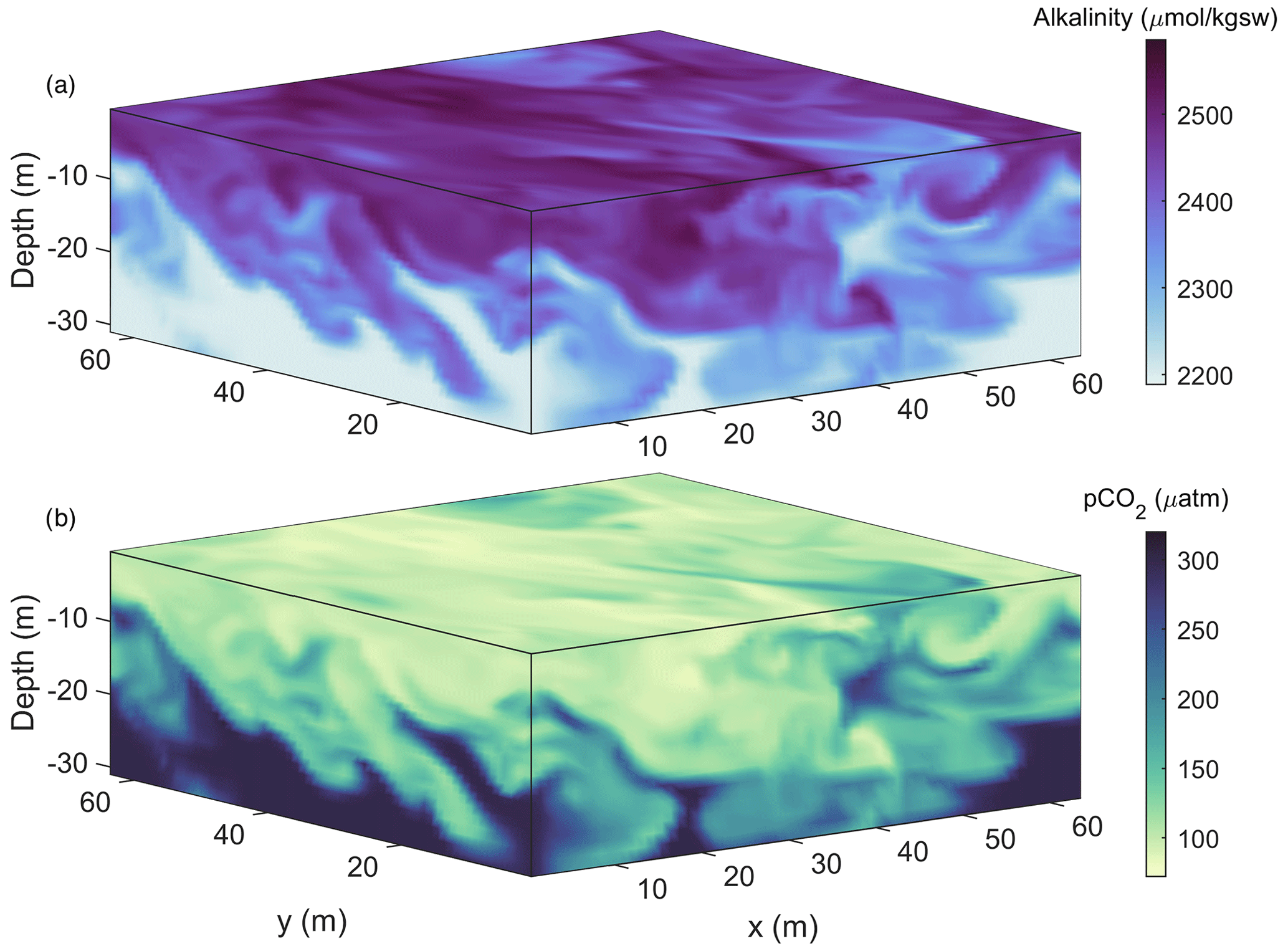
Figure 1LES of near-surface turbulence coupled to a carbonate system solver. Alkalinity is added at a rate of 4 µmol kg−1 m−2 s−1 for 20 min to the top grid cell at the start of the simulation. Turbulence, generated by surface wind stress and cooling, sets the rate at which it mixes downwards (a) along with associated waters of lowered pCO2 (b). Turbulent plumes and eddies lead to inhomogeneities in water properties at scales of tens of metres.
For alkalized plumes associated with outfalls from, for example, wastewater treatment plants, integral models (that assume plume properties such that the governing equations are simplified) have been developed to examine the initial dilution close to jets and buoyant plumes up to kilometre scales (Jirka et al., 1996). These models are highly configurable, enabling specific diffuser configurations as well as the potential to incorporate sediment-laden plumes with particle settling (Bleninger and Jirka, 2004). Results are commonly accepted for engineering purposes, defining mixing zones, and providing a fast “first look” at diffusion and mixing near an outfall site. However, these models rely on assumptions about the underlying physics of fluid flow (e.g., axisymmetric plumes and simplified entrainment rates) that may not be accurate under general oceanic conditions, and results will not include all effects of irregular bathymetry, finite domain size, or arbitrarily non-uniform ambient conditions. Nevertheless, their simplicity makes them very useful. For example, by combining several simple process models for plume dilution, particle dissolution, and carbon chemistry, Caserini et al. (2021) have simulated the initial dilution of slaked lime Ca(OH)2 particles and alkalinity in a plume behind a moving vessel.
Other methods for modelling at this scale include Reynolds-averaged Navier–Stokes (RANS) and unsteady RANS (URANS), wherein fluctuations against a slowly varying or time mean background are parametrized, often using constant (large-)eddy diffusivities and viscosities. These approaches are often inaccurate at these scales, resulting in simulations that are too diffusive or lacking processes that are of leading-order importance to mixing (Golshan et al., 2017; Chang and Scotti, 2004).
There are multiple, potentially interacting sources of uncertainty to consider when evaluating the uncertainty in the applications described above. Perhaps best understood but still problematic is the uncertainty that arises from the computational intractability of simulating all the relevant scales in the micrometre-to-kilometre range at once, necessitating the different modelling approaches for different scales, with parameterizations to account for unresolved scales and scale interactions. The dissolved carbonate chemistry of seawater is relatively well parameterized (Zeebe and Wolf-Gladrow, 2001), but some modest uncertainties arise from approximations required for computational tractability (Smith et al., 2018). The least understood but potentially dominant source of uncertainty pertains to the representation of the microscale biological, chemical, and physical dynamics of particles, which is an active area of experimental and observational investigation (Subhas et al., 2022; Fuhr et al., 2022; Hartmann et al., 2023). While the explicit multiphase modelling of the particles themselves is computationally costly, an approach wherein the parametrized evolution of inertia-less Lagrangian particles is simulated may provide a fruitful middle ground, providing a mechanism to realistically determine the alkalinity release field associated with the advection, mixing, sinking, and dissolution of reactive mineral particles. These questions about particles apply to those released in OAE deployments as well as particles that precipitate from seawater in part due to OAE deployments and finally the role of ambient biotic and abiotic particles where OAE is deployed.
2.1.2 Local to regional scales (metres to kilometres)
Local- to regional-scale models that range in horizontal resolution from tens of metres to hundreds of kilometres are useful for simulating the impact of alkalinity injections beyond the immediate local area, where conditions do not depend on the details of how the alkalinity was added and instead are determined by regional-scale currents and other process, including the potential for biogenic feedbacks. These models are particularly useful to support OAE field experiments, including planning and observational design as well as analysis, integration, and synthesis of observations, and to facilitate interpretation of observations from natural analogues. Furthermore, local- and regional-scale models will likely prove to be indispensable for quantification of OAE effects in research settings, for guiding assessments of its environmental impacts, and for MRV during the potential implementation of OAE. A skilful model can simulate when and where changes in carbonate chemistry and the ensuing anomalies in air–sea CO2 exchange occur and provide an estimate of the spatiotemporal extent of the biogeochemical properties affected by OAE.
Regional models have distinct advantages over global models in their ability to resolve the spatial scales on which OAE would be applied both experimentally and operationally and their documented skill in representing coastal and continental shelf processes more accurately (Mongin et al., 2016; Laurent et al., 2021). Examples of regional-model applications in the context of OAE include the recent studies by Mongin et al. (2021) and Wang et al. (2023). Mongin et al. (2021) used a coupled physical–biogeochemical–sediment model tailored to Australia's Great Barrier Reef to investigate the extent to which realistic OAE applied along a shipping line could alleviate anthropogenic ocean acidification on the reef. Wang et al. (2023) used a coupled ice–circulation–biogeochemical model of the Bering Sea to study the efficiency of OAE in coastal Alaska.
Implementation of a regional model in a target domain requires generation of a grid with associated bathymetry, specification of boundary conditions (including atmospheric forcing; information about ocean dynamics along the lateral boundaries of the domain; any fluxes of biogeochemical properties across the air–sea, sediment–water, and land–ocean boundaries; river inputs), and generation of initial conditions within the domain (Fennel et al., 2022). Different circulation models are available for implementation in domains targeted for OAE studies (see, e.g., Table 1 in Fennel et al., 2022), all with distinct strengths and established user communities. Particularly relevant in the context of studying coastal applications of OAE is a model's ability to accurately represent coastal topography, making unstructured grid models and models with terrain-following coordinates particularly attractive. Another feature to be considered is a model's ability to run in two-way nested configurations. In the more widely applied one-way nesting of domains, simulated conditions from a larger-scale model (referred to as the parent model) are used to generate the dynamic lateral boundary conditions of a smaller scale, higher-resolution model (the child model), which runs offline from the parent model. With two-way nesting, both models run simultaneously, and information is exchanged continually along their intersecting boundaries. This allows information generated within the high-resolution child domain (e.g., the spreading distribution of a tracer or alkalinity addition) to be received and propagated by the larger-scale parent model. In this context, model simulations are particularly useful if available in near-real time or in forecast mode. This requires specification of lateral boundary conditions and atmospheric forcing up to the present and into the future. Global ∘ nowcasts and 10 d forecasts of ocean conditions are available from the Copernicus Marine Service (CMEMS, 2023), and atmospheric forcings up to the present and 10 d into the future are available from the European Centre for Medium Range Weather Forecasts (ECMWF, 2023).
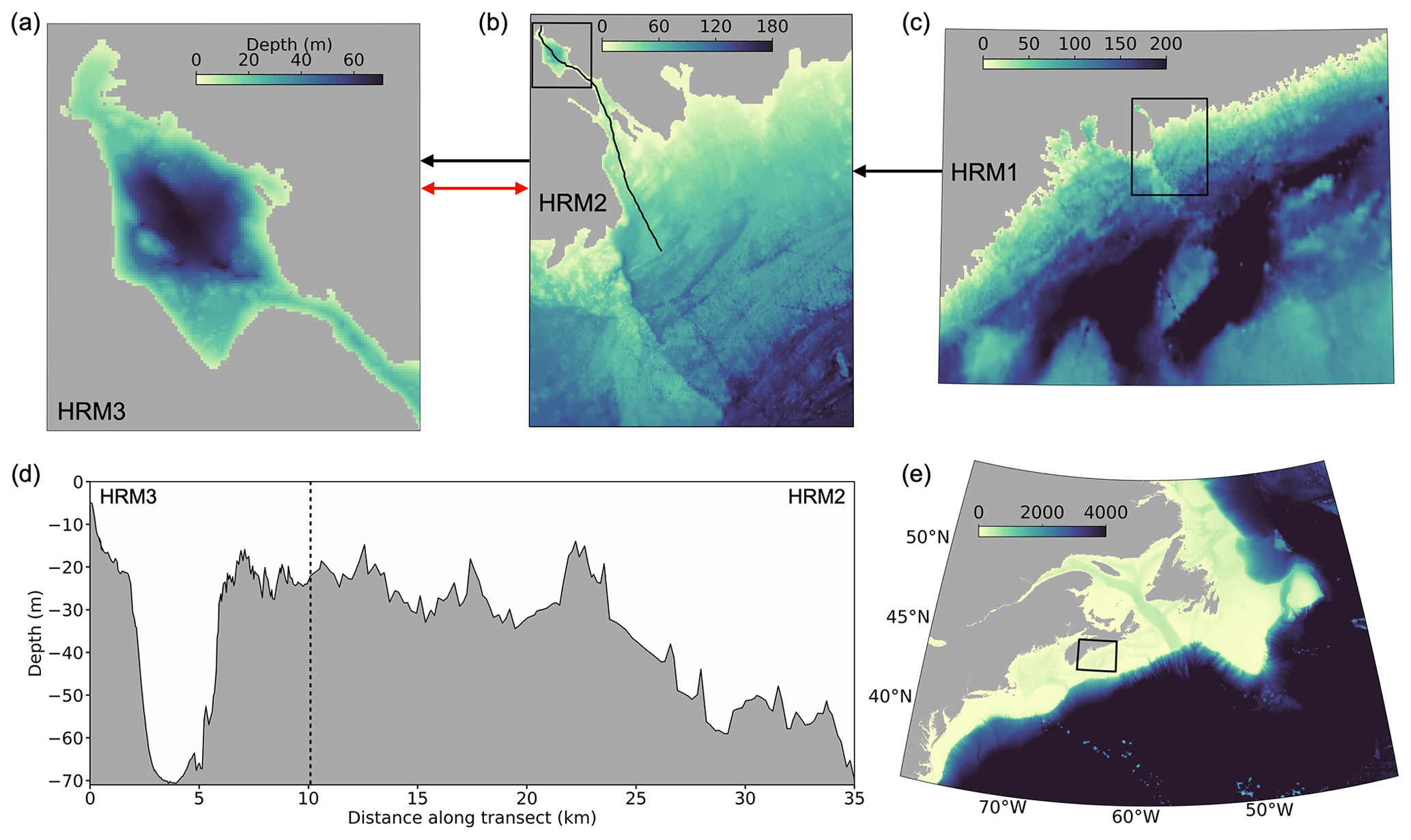
Figure 2Nested configuration of three ROMS models for the Bedford Basin and the adjacent harbour in Halifax Regional Municipality (HRM). (a) The highest-resolution model (HRM3, 60 m) includes the 7 km long and 3 km wide Bedford Basin and The Narrows, a 20 m shallow narrow channel that connects the basin to the outer harbour. (b) The larger-scale model (HRM2, 200 m) includes Bedford Basin and Halifax Harbour as well as the adjacent shelf. (c) The largest-scale model (HRM3, 900 m) covers the central part of the Scotian Shelf as indicated in (e). (d) Bathymetry along a section through HRM3 and HRM2, indicated by the black line in (b). Lateral boundaries of HRM3, HRM2, and HRM1 are shown by black boxes in (b), (c), and (e), respectively. Black arrows indicate the information flow between models in one-way nesting mode. The red arrow indicates that HRM1 and HRM2 can be run simultaneously with bi-directional flow of information (two-way coupled mode).
One example of a high-resolution local-scale model with two-way nested domains is a framework developed for Bedford Basin in Halifax, Canada (Fig. 2; Laurent et al., 2024). The model framework consists of three nested ROMS models (ROMS is the Regional Ocean Modelling System; Haidvogel et al., 2008; Shchepetkin and McWilliams, 2005). The outermost ROMS domain has a resolution of 900 m and is nested one-way within the data-assimilative GLobal Ocean ReanalYsis and Simulation (GLORYS) reanalysis of physical and biogeochemical properties (Lellouche et al., 2021). Nested within are two models with increasingly higher resolutions of 200 and 60 m. Depending on the scientific objective to be addressed, the models can be run in one-way and two-way nested mode, where two-way nesting is computationally more demanding, and in hindcast or forecast mode. Implementation of dye tracers within the model (Wang et al., 2024) allows one to determine dynamic distribution patterns and residence times.
2.1.3 The global scale
A strength of global ocean models is their capacity to comprehensively represent the global overturning circulation and ocean ventilation. These processes control the timescales over which waters are sequestered in the ocean interior and determine how long surface waters are exposed to the atmosphere and can exchange properties, including CO2, before being injected back into the ocean interior (Naveira Garabato et al., 2017). Similarly, the large-scale overturning circulation and the patterns associated with ventilation are important to consider in the context of deploying OAE at scale, as these patterns exert strong control on the efficiency of OAE at sequestering CO2 (e.g., Burt et al., 2021).
When global ocean models are dynamically coupled with models of the land biosphere and the atmosphere, they are referred to as Earth system models (ESMs) and can be employed to explore Earth system feedbacks to mCDR. In the case of OAE, the main feedback is the change in atmospheric pCO2 and air–sea gas exchange that will result when CDR approaches are implemented at scale. While regional models have to be forced by atmospheric CO2 concentrations, ESMs represent the atmospheric reservoir and are forced by CO2 emissions into the atmosphere, which then interacts with land and ocean carbon reservoirs. Only the latter approach can account for OAE-induced reductions in the atmospheric CO2 inventory, which, in turn, would lead to a systematic reduction in air–sea CO2 fluxes. Regional models and global ocean models that do not explicitly represent the atmospheric CO2 reservoir and instead are forced by prescribed atmospheric pCO2 cannot simulate the decline in atmospheric pCO2 due to OAE. Depending on the alkaline material applied, there may also be feedbacks associated with changes in temperature, albedo, nutrient cycles, and biological responses which can be studied with the help of ESMs.
Another important strength of global models relates to the fact that anomalies in air–sea CO2 flux generated by OAE deployments will manifest over large spatiotemporal scales because CO2 equilibrates with the atmosphere via gas exchange slowly. Alkalinity-enhanced waters can be transported far away from injection sites before equilibration is complete (He and Tyka, 2023). Consequently, OAE signals may exit the finite domain of regional models prior to full equilibration with the atmosphere (e.g., Wang et al., 2023). Because global models represent the entire ocean and can be integrated for centuries or longer, they enable full-scale assessments.
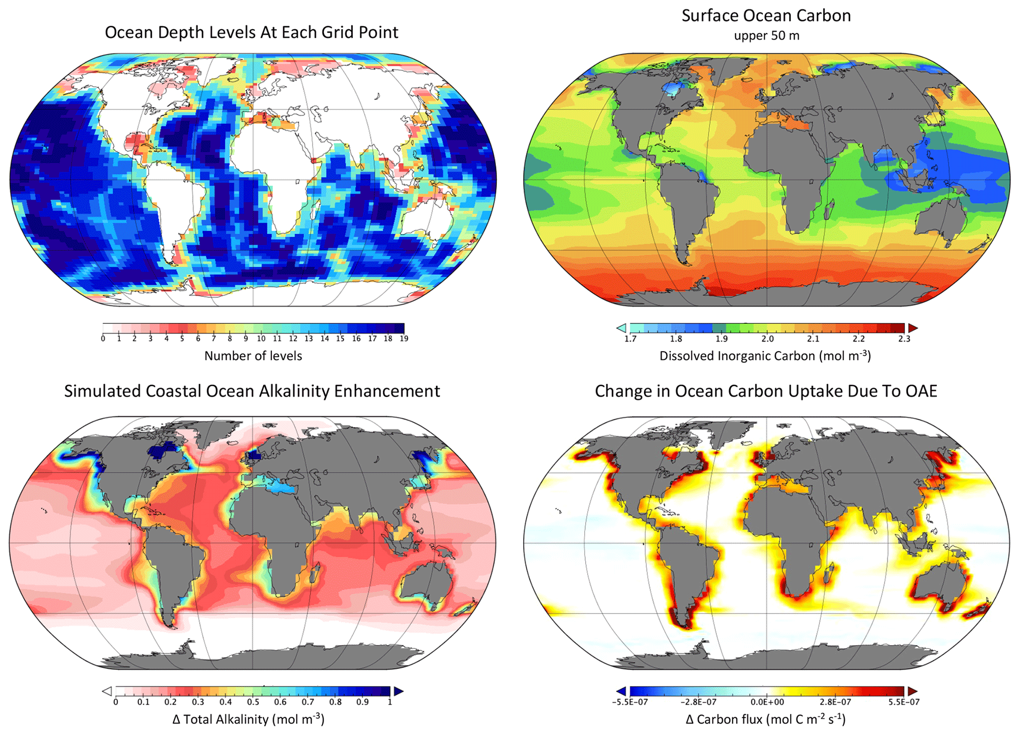
Figure 3Example of Earth system model properties and output from the University of Victoria Earth System Climate Model (Keller et al., 2012; Mengis et al., 2020) including (a) the model bathymetry (depth levels) and (b) the simulated present-day dissolved inorganic carbon concentration (mol m−3) averaged over the upper 50 m of the ocean. Panels (c) and (d) show results from a coastal OAE study by Feng et al. (2017), where the change in upper-ocean alkalinity (upper 50 m) and the air–sea flux of CO2 are shown relative to the Representative Concentration Pathway (RCP) 8.5 control simulation. The Oliv100_Omega3.4 simulation from Feng et al. (2017) is shown, where 100 µm olivine grains were added to ice-free coastal grid cells in proportion to RCP8.5 CO2 emissions (i.e., 1 mol of alkalinity per mole of emitted CO2) until a sea surface aragonite Ω threshold of 3.4 was reached.
A primary challenge for global models, however, is that their horizontal resolution is necessarily limited by computational constraints (see example in Fig. 3). Most of the global ocean models contributing to the Coupled Model Intercomparison Project version 6 (CMIP6), for example, have horizontal resolutions of about 1∘ or roughly 100 km (Heuzé, 2021) and do not accurately represent biogeochemical processes along ocean margins (Laurent et al., 2021). Model grid spacing imposes a limit on the dynamical scales that can be explicitly resolved in the models; this is particularly problematic for coarse-resolution global models because mesoscale eddies – i.e., motions on scales of about 10–100 km – dominate the variability in ocean flows (Stammer, 1997). Since coarse-resolution models cannot resolve mesoscale eddies explicitly, the rectified effects of these phenomena, including their role in transporting buoyancy and biogeochemical tracers, must be approximated with parameterizations (e.g., Gent and McWilliams, 1990).
Notably, the fidelity of the simulated flow in global models, including the imperfect nature of these parameterizations, projects strongly on the model's capacity to accurately simulate ventilation and the associated uptake of transient tracers, such as anthropogenic CO2 or chlorofluorocarbons (CFCs), from the atmosphere (e.g., Long et al., 2021). Biases in the uptake of transient tracers will also have implications for a model's capacity to faithfully represent the impact of OAE, where the path of alkalinity-enhanced waters parcels in the surface ocean, and their subsequent transport to depth is a key control on the efficiency of carbon removal. Biases in the simulated flow are also an important determinant of the simulated distribution of biogeochemical tracers in the model's mean state. Hinrichs et al. (2023), for example, demonstrate that inaccuracies in the physical redistribution of alkalinity by the flow is a dominant mechanism contributing to biases in the alkalinity distributions simulated by CMIP6 models.
Finally, another important challenge associated with global ocean models is the requirement to represent the entire global ocean ecosystem with a single set of model parameters (e.g., Long et al., 2021; Sauerland et al., 2019). In particular, the biological pump is an important control on the distribution of biogeochemical tracers, including alkalinity and dissolved inorganic carbon (DIC). The magnitude of organic carbon export and the magnitude of biogenic calcium carbonate export are important controls on the distribution of alkalinity and DIC at the ocean surface and in the interior (e.g., Fry et al., 2015). These quantities are a product of ecosystem function and, since the global ocean is characterized by diverse biogeography (e.g., Barton et al., 2013), capturing global variations in the biological pump presents a challenge.
2.1.4 Integration across scales
Choosing the appropriate modelling tool for a given OAE-related question requires clarity about the scale of the problem to be addressed and the objectives of the model application. Approaches for OAE vary significantly with respect to the spatial footprint of alkalinity increase. Proposed methods for spreading alkalinity feedstocks at the surface ocean include the addition of reactive minerals (e.g., CaO, Ca(OH)2, or Mg(OH)2) in ship-propeller washes (e.g., Köhler et al., 2013; Caserini et al., 2021) or using other means (e.g., Gentile et al., 2022) along tracks from commercial or dedicated OAE vessels or through coastal outfalls (e.g., wastewater treatment or power plants); the addition of less-reactive minerals to corrosive or high-weathering environments (e.g., olivine spreading on beaches or mineral addition to riverine discharge; e.g., Montserrat et al., 2017; Foteinis et al., 2023; Mu et al., 2023); and electrochemically generated point sources of alkalinity that are discharged as highly alkaline seawater (e.g., House et al., 2009) from existing facilities (e.g., desalination and wastewater treatment plants), dedicated facilities (e.g., Wang et al., 2023), or an array of smaller infrastructure (e.g., grids of offshore wind turbines). Models for OAE research should represent these footprints of alkalinity increases appropriately for the questions being addressed.
There are research questions that fall relatively neatly into one of the three scale ranges described above in Sect. 2.1.1 to 2.1.3. For example, consideration of the near-field effects of different alkalinity feedstocks (e.g., dissolved versus particles) or analysis of the potential impacts from secondary CaCO3 precipitation due to elevated alkalinity from a point source requires models that resolve the scales of turbulent motion. Examination of the change in air–sea CO2 flux due to a broad and diffuse alkalinity increase is less demanding on model resolution, and regional-scale models are appropriate for this question. Investigation of Earth system feedbacks requires ESMs. However, there are also many aspects of OAE that require a bridging of scales. For example, when considering different deployment methods like discharge from vessels into the ocean surface boundary layer versus additions made through outfalls via surface or subsurface plumes, modelling requirements vary. In both cases, the resulting biogeochemical response may be affected by dynamics operating in the near field, where conditions are sensitive to the deployment method, and turbulence has to be considered, and the far field, where conditions do not depend on the details of how the alkalinity was added, and the air–sea flux of CO2 is instead determined by ambient environmental processes. Another example is the challenge that anomalies in air–sea CO2 flux generated by OAE deployments will manifest over large spatiotemporal scales because CO2 equilibrates with the atmosphere via gas exchange slowly. Some interplay among the modelling tools described in Sect. 2.1.1 and 2.1.2 is likely going to be required. One straightforward approach would be to parameterize small-scale processes in the larger-scale models.
2.2 The range of biogeochemical realism and complexity
Application of biogeochemical ocean models for the purposes of OAE research and verification requires re-evaluation, and likely further development, of several model assumptions and features related to biogeochemical realism and complexity. For example, the internal sources and sinks of alkalinity are typically not explicitly represented in ocean models; this may become necessary in some circumstances but will be challenging (Sect. 2.2.1). OAE-related perturbations of alkalinity and other carbonate system properties and addition of macro- and micronutrients contained in some alkalinity feedstocks may result in biological and ecosystem responses that current biogeochemical models are not capable of representing but that would be relevant for the assessment of environmental impacts of OAE and the verification of its CDR efficiency (Sect. 2.2.2). Furthermore, depending on the environmental setting, sediments can be sources or sinks of alkalinity; these sediment–water fluxes need to be appropriately considered, including the potential impacts of OAE on their magnitude, in order to obtain complete and trustworthy carbon budgets (Sect. 2.2.3). Other boundary fluxes that require accurate specification are alkalinity inputs from rivers and groundwater (Sect. 2.2.4) and the air–sea flux of CO2 across the air–sea interface (Sect. 2.2.5).
2.2.1 Representing alkalinity in seawater
Alkalinity is an emergent property that depends on the concentrations of numerous chemical species with distinct internal sources and sinks (Schulz et al., 2023, this Guide; Wolf-Gladrow et al., 2007; Middelburg et al., 2020). Skilful simulation of alkalinity in seawater may require explicit representation of its multiple biotic and abiotic sources and sinks, some of which are difficult to constrain. A major process by which alkalinity is consumed is the production of calcium carbonate. In the water column, this is predominantly a biotic process, performed by calcifiers, although “whiting” events, where calcium carbonate precipitates spontaneously from ambient seawater, can be locally important (e.g., Long et al., 2017).
Models vary in the degree of mechanistic sophistication with which biogenic calcification is represented. For example, some models explicitly resolve calcifiers, such as pelagic coccolithophores (e.g., Krumhardt et al., 2017) and foraminifera (Grigoratou et al., 2022) and, in some cases, also benthic corals, foraminifera, or calcifying higher trophic levels, and thus can mechanistically account for the associated alkalinity consumption. Alternatively, models can parameterize biotic production of carbonate and its subsequent sinking and dissolution, as a fraction of organic matter production combined with an assumed remineralization profile (e.g., Schmittner et al., 2008; Long et al., 2021). Dissolution of carbonate minerals produces alkalinity at the sediment surface and in the water column as carbonate particles sink. This can be represented with first-order abiotic dissolution kinetics with a dependence on the saturation state of ambient water in the water column (e.g., Sulpis et al., 2021); in the sediments (e.g., Emerson and Archer, 1990); or in micro-environments in aggregates or organisms (Barrett et al., 2014) with systematic differences for different crystal structures such as aragonite and calcite (Morse et al., 1980).
Production of alkalinity occurs via uptake of nitrate or nitrite by photoautotrophs, while remineralization consumes alkalinity when happening aerobically but generates alkalinity when occurring anaerobically, e.g., via denitrification (Fennel et al., 2008). Biotic production and consumption of alkalinity is stoichiometrically coupled to the release or uptake of nutrients and carbon, where non-Redfield processes such as nitrogen fixation or denitrification need to be specifically considered in the stoichiometric relationships (Paulmier et al., 2009).
Spontaneous precipitation of carbonate minerals in pelagic environments could occur when seawater is highly oversaturated with respect to carbonate (Moras et al., 2022) but is, to the best of our knowledge, not yet included in ocean models. When simulating OAE approaches that may generate high oversaturation with respect to carbonate, spontaneous precipitation of carbonates needs to be considered, especially when condensation nuclei are present. Appropriate approaches will have to be developed, e.g., using near-field models to mechanistically represent this process and a meta-model approach to develop parameterizations that are suitable for far-field and larger-scale models.
Organic compounds produced within the ocean or originating from land can also act as proton acceptors and contribute to organic alkalinity (e.g., Koeve and Oschlies, 2012; Ko et al., 2016; Middelburg et al., 2020) and will impact the carbonate system, the partial pressure of CO2, and thus the air–sea CO2 flux. Commonly, the contribution of organic alkalinity is deemed small enough in oceanic environments to be negligible, but this assumption should be reconsidered in the context of OAE, especially for coastal CDR deployments where the organic contribution to alkalinity is thought to be larger. To the best of our knowledge, models do not account for organic alkalinity. A better quantitative understanding of organic contributions to alkalinity is likely needed to parameterize or mechanistically represent its contribution in models. Similarly, it may be important in the context of mineral OAE deployments to account for local variations in [Ca2+] and [Mg2+] to accurately estimate the pCO2 anomalies generated by different OAE feedstocks. While these constituents have very long residence times in the ocean and are hence commonly assumed to vary conservatively in proportion to salinity, variations in their relative abundance has an impact on the thermodynamic equilibrium coefficients used to solve seawater carbonate chemistry (Hain et al., 2015).
2.2.2 Representing biological and ecological processes
A key question related to OAE is whether changes in carbonate chemistry induce differential responses in organisms. In the pelagic zone, OAE might shift the phytoplankton community composition, for example, due to distinct physiological sensitivities of different groups (e.g., Ferderer et al., 2022). Further, if OAE is accomplished via rock dissolution, carbonate versus silicate rock may impact the relative balance between phytoplankton functional groups (PFTs) such as calcifiers and diatoms, and changes in Mg and Ca ratios may also influence calcification (Bach et al., 2019). Additionally, ancillary constituents specific to particular feedstocks may have biological activity. Silicate rocks include bioreactive metals such as Fe, a micronutrient with the capacity to stimulate phytoplankton growth, and others that can be toxic when occurring in high concentrations, such as Ni and Cu, and may adversely impact phytoplankton and reduce primary productivity (Bach et al., 2019). The bioreactivity of these metals may be difficult to simulate in models as their dissolved concentrations can be partially mediated by complexation with organic ligands (Guo et al., 2022). Physical impacts of OAE feedstocks may also have important biological impacts through changes in the propagation of light in the surface ocean, and direct exposure to mineral particles may have additional impacts, e.g., on zooplankton through particle ingestion (Harvey, 2008; Fakhraee et al., 2023). Effects of OAE on plankton have the potential to propagate to higher trophic levels through marine food webs as the magnitude and quality of net primary productivity shifts, and trophic energy transfer is altered accordingly.
Simulating this full collection of processes in models is challenging. Dominant modelling paradigms for simulating planktonic ecosystems include PFT- and trait-based models (e.g., Negrete-Garcia et al., 2022). In these systems, physiological sensitivities are parameterized according to transfer functions that modulate rate processes – growth, for instance – on the basis of ambient environmental conditions. Nutrient limitation of growth is often represented using Michaelis–Menten kinetics wherein growth rates decline as nutrient concentrations become limiting. State-of-the-art ESMs represent PFTs with multiple nutrient co-limitation, which is essential to effectively simulate plankton biogeography of the global ocean. Diatoms, for example, are capable of high growth rates, enabling them to outcompete other phytoplankton under high-nutrient conditions, but their range is restricted to high latitudes and upwelling regions where there is sufficient silicate. If OAE were to modulate the concentration of constituents represented by multiple nutrient co-limitation models, it is possible such models could simulate the phytoplankton community response – though it is important to consider whether the models provide representations that are sufficiently robust for the magnitude of OAE-related perturbations. In some cases, models are missing key processes that would be required to mechanistically simulate certain effects. We are aware of no models that represent Ni toxicity, for instance. Including these effects, as well as a capacity to simulate secondary interactions, such as ligand complexation of metals in OAE feedstocks, will require significant investment in empirical experimentation to understand essential rate processes and physiological responses.
Shortcomings in the capacity of models to represent physiological responses to OAE is an important consideration for the ability of models to faithfully represent ecological impacts. Notably, electrochemical OAE techniques present a simpler set of processes to consider than using crushed-rock feedstocks, where ancillary constituents and physical dynamics come into play. For electrochemical OAE, the most likely biological feedback to consider relates to the impacts of changing carbonate chemistry on biogenic rates of calcification or phytoplankton growth rates (Paul and Bach, 2020). It is also possible that carbon limitation of phytoplankton growth (Paul and Bach, 2020; Riebesell et al., 1993) may also be important. Empirical research exploring physiological sensitivities should be used to develop prioritizations of key model processes comprising early targets for implementation. Model documentations should use consistent stoichiometric relations to link alkalinity changes to those of nutrients and carbon (Paulmier et al., 2009) and state the assumptions made about carbonate formation and dissolution.
2.2.3 Representing sediment–water exchanges
The exchange of solutes between the sediments and overlying water influences ocean chemistry, including the properties of the carbonate system (Burdige, 2007). Depending on location and timescale, OAE may affect these exchanges and should be appropriately considered in models. Sediments influence the marine carbonate system primarily through the remineralization of organic matter, which returns DIC to overlying water (and alkalinity if this remineralization occurs anaerobically), and the dissolution of biogenic silicate or carbonate minerals. CaCO3 is of particular importance as its dissolution releases alkalinity, while its burial is an alkalinity sink, and the balance between the two is a key control on the ocean's alkalinity balance over timescales approaching 104 years (Middelburg et al., 2020). Furthermore, remineralization and other microbial metabolisms, such as “cable bacteria,” can significantly lower pore water pH by several pH units below seawater values (Meysman and Montserrat, 2017). This can drive dissolution of CaCO3 and generate alkalinity in the sediments, even in shallow waters when the overlying water is supersaturated (Rau et al., 2012).
Representing these processes in coastal and shelf sediments (< 200 m) is challenging. Shallow water depths and high productivity result in a significant delivery of organic matter to the sediments that is much larger than in the deep ocean. As a result, the relative importance of sediments in organic matter remineralization is larger, and production of alkalinity by anaerobic metabolisms is more important in these shallow sediments than in the deep ocean (Seitzinger et al., 2006; Jahnke, 2010; Huettel et al., 2014; Chua et al., 2022). In addition, these environments are dynamic, with organic supply and bottom water conditions varying on tidal, seasonal, and interannual timescales. Accounting for the exchange between sediments and overlying water and its variability on tidal, seasonal, and interannual timescales will likely be necessary in regional and global biogeochemical models that aim to simulate alkalinity cycling in coastal and shelf seas, even for relatively short simulation durations of months to years.
The choice of approach to modelling sediments may depend on the sediment type. For example, the mechanisms transporting solutes across the sediment–water interface can be divided into two categories depending on the sediment's grain size. In coarse sediments, i.e., permeable sands, pressure gradients drive flow through the seabed, replenishing sediment oxygen content (Huettel et al., 2014). Organic carbon stores are low, and remineralization was long thought to be primarily aerobic. However, evidence has emerged relatively recently that anaerobic remineralization in sandy sediments is more important than originally thought (Chua et al., 2022, and references therein). Idealized models that represent the three-dimensional sediment structure illustrate the importance of turbulence and oscillatory flows in permeable sediments (see Box 2 in Chua et al., 2022). These models are highly localized and computationally demanding, prohibiting their coupling with ocean biogeochemical models. Thus, permeable sediments are currently not well represented in regional or global ocean biogeochemical models.
In cohesive, fine-grained sediments with low permeability, i.e., muds, transport is limited by diffusion or faunal-mediated mixing and exchange processes, i.e., bioirrigation or bioturbation (Meysman et al., 2006; Aller, 2001). In these environments, detailed multicomponent reactive-transport models of sediment biogeochemistry – so called diagenetic models – can reproduce carbon remineralization rates partitioned between aerobic and anaerobic pathways, precipitation/dissolution reactions between sediment grains and porewaters, and the transport of solutes across the sediment–water interface (Boudreau, 1997; Middelburg et al., 2020). These mechanistic models will be useful for detailed investigations into how perturbations of the carbonate system in seawater overlying the sediments affect their biogeochemistry and for addressing questions about the potential influence of particulate alkalinity feedstocks settling to the seafloor (Montserrat et al., 2017; Meysman and Montserrat, 2017). However, typically these models are one-dimensional and applied to a few representative locations. Coupling fully explicit diagenetic models to three-dimensional ocean biogeochemical models, while conceptually straightforward, is computationally prohibitive. Instead, depth-integrated sediment processes have been implemented as bottom boundary conditions (e.g., Moriarty et al., 2017, 2018; Laurent et al., 2016). For example, Laurent et al. (2016) used a diagenetic model in a “meta-modelling” approach to estimate bottom boundary nutrient fluxes for a regional-scale biogeochemical model. By parameterizing the diagenetic model with detailed geochemical data (porewater profiles and nutrient fluxes) from a few individual locations, then forcing it over a range of expected bottom water conditions, they developed empirical functions relating sediment fluxes to bottom water conditions that could be used to parameterize bottom boundary conditions in the water column model. A similar approach could be used in OAE models to parameterize how sediment biogeochemistry may alter alkalinity fluxes, for example, how redox sensitive processes, such as coupled nitrification–denitrification or sulfate reduction coupled to pyrite burial, both of which may produce alkalinity (Soetaert et al., 2007), may respond to changes in bottom water oxygen or organic matter loading.
When considering the long-term storage of CO2 in global-scale ESMs, the interactions between sediments and the deep ocean (> 1000 m bottom depth) may need to be considered. In this environment most organic matter remineralization occurs in the water column, and the small amount of organic matter reaching the seafloor is remineralized aerobically with little to no release of alkalinity. In this case, sediment remineralization can likely be either ignored or implemented as a reflective boundary condition where the simulated particulate organic carbon (POC) flux to the seafloor is immediately returned as DIC and remineralized nutrients. However, the dissolution or preservation of CaCO3 in deep sediments is critical to controlling deep-water alkalinity and may be important in model simulations that aim to quantify OAE effects on the timescales associated with the large-scale global overturning circulation. CaCO3 solubility increases with pressure and decreasing pH, and CaCO3 eventually becomes undersaturated at depth. The depth at which sinking CaCO3 balances its dissolution is referred to as the carbonate compensation depth (CCD). An increase in bottom water CO or CaCO3 deposition will deepen the CCD, burying CaCO3, trapping alkalinity, and lowering the alkalinity budget of the ocean. Conversely if CaCO3 rain rate or CO concentration decreases, the CCD will shoal, and previously buried CaCO3 will dissolve, releasing alkalinity to the deep ocean. CCD compensation therefore opposes any forcing of the deep ocean carbonate system and therefore dampens the rise in CO2 in the atmosphere but will also counteract any potential OAE solution (see Renforth and Henderson, 2017, for a detailed explanation). Although most CaCO3 dissolution occurs in the sediments, there is no consensus as to the level of detail this needs to be represented in models. Some global models employed to investigate large-scale OAE include calcium carbonate dynamics at the sediment surface (Ilyina et al., 2013); others disregard this process (Keller et al., 2014).
Often global models will parameterize CaCO3 burial as a function of saturation state. Such an approach is effective for resolving CCD dynamics over geological timescales (∼ 10 000 years), but not over the century to millennial timescales of CCD readjustment. Models that fully couple sediment diagenesis can resolve these dynamics (Gehlen et al., 2008), but the computational demand can make them ineffective. One solution is the approach of Boudreau et al. (2010, 2018). By suggesting that CaCO3 dissolution dynamics are controlled by transport of dissolution products across the benthic boundary layer, they were able to derive equations predicting CCD depth and CaCO3 dissolution based on bottom water CO and CaCO3 rain rate and avoiding a detailed representation of the sediments. These equations, combined with model bathymetry, can parameterize sediment CO flux as a boundary condition and suitably account for transient sediment CaCO3 dissolution in large-scale ESMs while avoiding the computational demands of a fully coupled ocean circulation–diagenesis model.
2.2.4 Representing river and groundwater fluxes
Regional and global ocean biogeochemical models typically account for river inputs, including their contributions to alkalinity and DIC. In most models this is done by specifying alkalinity and DIC concentrations in imposed riverine freshwater fluxes, although accurate prescription of these concentrations can be challenging. Typically, a combination of direct river measurements where available, output from watershed models (e.g., Seitzinger et al., 2010), and extrapolations of coastal ocean measurements to a freshwater endmember (e.g., Rutherford et al., 2021) is used. Solute inputs from groundwater are typically ignored but could be important locally. In high-resolution coastal domains near urban areas, sewage input may be an additional important source of carbon, nutrients, and alkalinity.
It is important to note that land-based CDR applications may have an important effect on ocean alkalinity dynamics through riverine and groundwater delivery of solutes. Terrestrial OAE equivalents broadly referred to as enhanced rock weathering (ERW) rely on the application of lime or pulverized silicate or carbonate rocks on land and in rivers. These strategies aim to generate CO2 uptake locally but yield a leaching flux of bicarbonate into freshwater systems and subsequent transport into the coastal ocean. Field trials and some commercial applications are currently underway, most of them with the implicit or explicit assumption that the enhanced delivery of alkalinity will generate carbon removal in the ocean (Köhler et al., 2010; Taylor et al., 2016; Bach et al., 2019). There is a need for coordinated efforts to improve quantification of background riverine fluxes and establish initiatives to effectively track the solute additions from ERW.
2.2.5 Representing air–sea gas exchange
The calculation of air–sea gas exchange is necessary for the quantification of net carbon uptake from OAE in models. Biogeochemical models typically represent this exchange using a bulk relationship that depends on the product of the gas transfer velocity and the effective air–sea concentration difference (Fairall et al., 2000). However, the gas transfer velocity remains highly uncertain and is sensitive to a collection of processes that vary across scales, including sea state, boundary layer turbulence, bubble dynamics, and concentrations of surfactants. The most widely used parameterizations of the gas transfer velocity use empirical fits to observations to construct a functional relation dependent on wind speed only, under the premise that turbulence and bubbles (via the breaking of surface gravity waves) are predominantly determined by wind stress (Wanninkhof, 2014). This neglects processes that could be regionally important such as convection, modification by biological surfactants, rain, and wave–current interactions while vastly simplifying the effects of wave breaking and bubbles. Although different dependencies on wind speed have been proposed (quadratic, cubic, hybrid), parameterizing the gas transfer coefficient as a quadratic function of the 10 m wind speed is the most common (Wanninkhof, 1992, 2014). This relationship is supported by direct measurements of air–sea flux at intermediate wind speeds (3–15 m s−1), but at low wind speeds (< 3 m s−1), non-wind effects can have an important impact on gas transfer. At high wind speeds (> 15 m s−1), breaking waves and bubble injection enhance gas exchange for lower-solubility gases such as CO2 (Bell et al., 2017). Therefore, quadratic fits tend to underestimate the gas exchange at low and high wind speeds (Bell et al., 2017).
More complex air–sea exchange parameterizations account for processes such as bubbles, near-surface gradients, and buoyancy-driven convection (e.g., Liang et al., 2013; Fairall et al., 2000), but they depend upon a wider range of input variables. Other considerations in estimating flux arise from the nonlinear dependence on these variables, e.g., wind speed, which can lead to underestimates when made using daily averages rather than hourly measurements (Bates and Merlivat, 2001).
Notably, the gas transfer velocity (kw) determines the kinetics of gas exchange, given a perturbation in surface ocean pCO2 away from equilibrium. The timescale for CO2 equilibration over the surface mixed layer can be fully quantified using the following expression:
where h is the depth of the surface mixed layer, and the partial derivative captures the thermodynamic state of the carbon system chemistry in seawater, specifically with respect to the amount that dissolved CO2 changes per unit change in DIC (Sarmiento and Gruber, 2006). This property is related to the buffer capacity and varies in roughly linear proportion to the carbonate ion concentration. The magnitude of is typically about 20, which explains why the equilibration timescale for CO2 is so long. The contribution of uncertainty in the gas exchange velocity to overall uncertainty in carbon uptake from OAE deployments will depend in part on the circulation regime involved. For example, in situations where alkalinity-enhanced water parcels are retained at the surface for timescales that are significantly longer than τgas-ex, full equilibration will occur, and the impact of uncertainty in the gas exchange velocity will have limited influence on the overall uncertainty.
Even though OAE-induced additional air–sea CO2 fluxes will, even in hypothetical massive deployments, amount to at most a few gigatonnes of CO2 per year, which is typically not more than 1 % of the atmospheric CO2 inventory, this subtle difference in the treatment of the atmospheric boundary condition can be significant. Using prescribed atmospheric pCO2 that is unresponsive to marine CDR-induced air–sea CO2 fluxes has been shown to overestimate oceanic CO2 uptake by 2 %, 25 %, 100 %, and more than 500 % on annual, decadal, centennial, and millennial timescales, respectively (Oschlies, 2009). Simulations with prescribed atmospheric pCO2 need to take such systematic biases into account.
2.3 Model development needs for OAE research
While there is already substantial capacity for simulating ocean biogeochemical dynamics at global to regional scales, the discussion above implicates several areas where additional efforts are required to fully establish a modelling capability suitable for supporting OAE. These fall into four primary areas: (1) supporting multiscale simulations with sufficiently high-fidelity flow fields, (2) faithfully simulating the near-field dynamics associated with alkalinity addition, (3) capturing feedbacks to OAE owing to biological and geochemical responses, and (4) identifying whether there are reduced-complexity modelling approaches that might provide sufficiently robust estimates of the net effects of OAE.
As elucidated above, a primary consideration related to capturing OAE impacts is the fidelity of the simulated flow. Notably, OAE presents a somewhat novel use case requiring an effective multiscale modelling capability. A conceptually straightforward path to improving the representation of ocean circulation and mixing is to increase the resolution of the model grid. However, the computational demand of high-resolution simulations can only be met over more limited-area domains. Since the spatiotemporal footprint of OAE-related perturbations is likely to be large, there will be a need to represent large regions. An argument might be made, however, that the circulation in proximity of an OAE site is most important to capture with high-fidelity. This can be achieved with two-way nested regional models as described in see Sect. 2.1.2 but will require further development to couple in the near-field models described in Sect. 2.1.1. Native grid refinement, e.g., via unstructured grids, is another approach that may be pursued to effectively support OAE research.
The second area of model development relates to the requirement of faithfully representing the dynamics associated with alkalinity addition. Regional to global scales are the most relevant for simulating the air-to-sea exchange of CO2 ensuing from OAE. It is important, however, to ensure that local processes affecting the mass fluxes and initial dispersal of alkalinity are handled appropriately. As illustrated above, DNSs or LESs (Sect. 2.1.1) can be leveraged to develop parameterizations for larger-scale models, including for crushed-rock feedstocks, where particle dynamics may be important, or techniques involving alkalinity-enhanced streams entering the ocean from outfall pipes. In addition to process fidelity, there are also numerical constraints to consider. For example, advection schemes used in most ocean general circulation models struggle to represent sharp gradients; large mass fluxes of alkalinity into single model grid points are likely to cause advection errors that may contaminate aspects of the model solutions, making interpretation difficult. More specifically, conservative advection schemes can be characterized in terms of their accuracy, monotonicity (i.e., ability to preserve sign), and linearity (i.e., ability to preserve additivity), and there are always tradeoffs to make between these properties. Research may be required to determine which schemes are best suited to the particular challenges associated with representing the advection of OAE signals.
The third area of model development relates to our capacity to fully capture the range of biogeochemical feedback associated with OAE. The class of processes to consider here is potentially large, and many have been touched on in Sect. 2.2.1 to 2.2.3. Precipitation dynamics, specific elemental components of alkalinity, biogenic responses mediated by physiological or ecological sensitivities, impacts and processes controlling the cycling of ancillary constituents, and accurate sediment–water exchange are all areas that merit consideration. Further efforts are required to understand and prioritize these areas of potential development, and, notably, their relative importance is likely to be regionally dependent.
Finally, it is important that models be tailored to address specific questions of relevance. In this context, it may be important to consider how much model complexity is required to capture the effects of perturbations, seeking parsimonious representations that are well supported by empirical constraints and invoking wherever possible a separation of concerns to isolate the factors contributing to uncertainty. For example, there are several near-field considerations that might be addressed using a combination of local observations and ultra-high-resolution modelling tools to generate estimates of alkalinity mass fluxes that are subsequently imposed as forcing in regional- to global-scale models. Another key question is how important it is to comprehensively simulate the mean state to faithfully capture the response to OAE perturbations for the purpose of MRV. For example, if it can be documented that biological feedbacks to OAE are of negligible concern, the core target for simulating OAE effects for MRV may be to capture the cumulative integral of air–sea CO2 exchange associated with the induced surface ocean pCO2 anomaly. The mean state of the seawater carbon system is relevant here as the background DIC and alkalinity fields determine the pCO2 response per unit addition of alkalinity, but fully prognostic calculations of nutrient cycling may not be necessary.
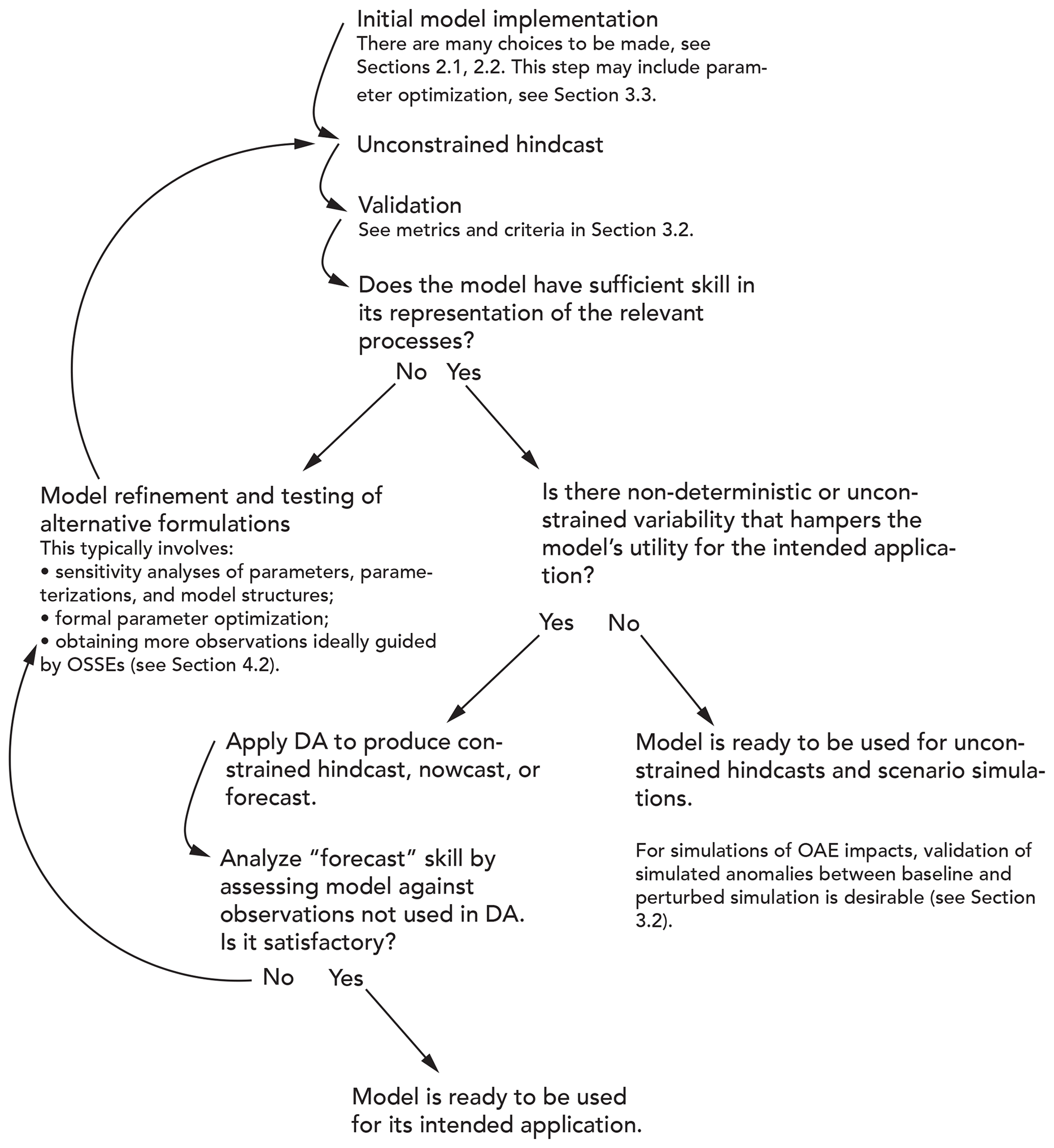
Whether a model is useful for OAE research depends on how accurately it represents the physical, chemical, and biological processes that are relevant to the specific research question to be addressed. Model validation, the evaluation of a model's performance, and estimation of uncertainties in model output should thus be integral parts of model implementation and application. It is important to note that any model, even after best efforts have been made to improve formulations and conduct the most thorough validation, will deviate from reality. Any model is, by definition, a simplification of the real world, and thus its output will be subject to uncertainties. Deviations of the model state from the real world can be reduced by applying statistical techniques, collectively referred to as data assimilation (DA) methods, that combine models with observations and yield the best possible estimates. The steps typically involved in model implementation and validation and possible integration with observations through data assimilation are shown in Fig. 4. In this section, we summarize the most important observation needs for model validation (Sect. 3.1), briefly describe typical metrics for model validation and articulate a reasonable minimum criterion (Sect. 3.2), give a high-level explanation of approaches for the formal statistical combination of models with observations through parameter optimization and state estimation (Sect. 3.3), and describe approaches for the specification of uncertainty in model outputs (Sect. 3.4).
3.1 Observation types for validation
Two fundamental requirements for models to be useful in the context of OAE research are high-fidelity representations of physical transport due to advection and mixing and of biogeochemical effects of OAE and most importantly changes in the inorganic carbon properties.
Observations for validation of the simulated physical transport of alkalized waters include temperature and salinity distributions, direct measurements of currents, surface drifter trajectories, sea surface height observations from satellite altimetry, and estimates of geostrophic flow derived from the latter. Additional metrics relevant for assessing the fidelity of the large-scale overturning circulation in global models include combinations of biogeochemical concentration and transient tracers. For example, oxygen can be useful for identifying large-scale transport pathways, even though it convolutes dynamical and biological information. Particularly valuable for assessing large-scale ocean transport on the timescales relevant for OAE are abiotic transient tracers such as chlorofluorocarbons (CFCs), sulfur hexafluoride (SF6), and possibly the isotopes 39Ar and 14C. Observational approaches for validation at regional scales include explicit tracer studies for documenting dispersion properties using Rhodamine dye or SF6.
In addition to the dynamics of the flow, model validation for OAE research requires the assessment of the fidelity of simulated carbonate chemistry variables (e.g., alkalinity, total DIC, pH, pCO2) and salinity and temperature, which are used to calculate the 13 thermodynamic equilibrium constants and conservative chemical species needed to constrain seawater acid–base chemistry in oxygenated seawater. Depending on the OAE approach and the model application, assessment may also require observed macronutrient (e.g., nitrate, silicate, or phosphate), micronutrient (e.g., Fe), and contaminant (e.g., Ni and Cr) measurements; bulk seawater properties related to biogeochemical cycling (e.g., dissolved organic carbon content, DOC; particulate inorganic carbon, PIC; chlorophyll fluorescence); and biogeochemical rates and fluxes (e.g., net community calcification).
It is not always feasible to obtain the ideal carbonate system observations for model validation. Temperature and salinity can be measured reliably across all ocean depths and, with greater uncertainty and only at the ocean surface, remotely from satellites. The technical capacity for seawater pH measurements is evolving rapidly, and sensors and systems now exist for pH measurements across nearly all depths, though the depth-capable systems require regular recalibration (e.g., Maurer et al., 2021). Similarly, there are numerous ways to observe surface ocean pCO2 using a variety of crewed, autonomous, and fixed-location platforms (e.g., ship-based, Saildrone, and moored systems). However, interior-ocean pCO2 observations remain challenging to obtain due to the need for calibration gases and a gas–water interface. Alkalinity titrations are predominantly performed on discrete bottle samples collected by hand, though autonomous titration systems are under development that enable in situ surface time series measurements (Shangguan et al., 2022). Microfluidic in situ alkalinity titrators are also under development that consume less reagent per sample but currently show higher uncertainties than discrete samples (Sonnichsen et al., 2023). Solid-state titrators that generate acid titrant in situ show promise for surface and subsurface alkalinity titrations, but these sensors are still undergoing development and validation (Briggs et al., 2017). DIC observations combine the limitations of current measurement systems for both the pCO2 and alkalinity, and there are only a handful of automated DIC titration systems rated for surface ocean measurements (e.g., Fassbender et al., 2015; Wang et al., 2015; Ringham, 2022). Theoretically, measurement of two of the carbonate system parameters in combination with temperature and salinity and some additional assumptions allows calculation of the other carbonate system parameters in seawater. Unfortunately, the pair of pCO2 and pH, which are the most accessible to autonomous measurement among the carbonate system parameters, provide nearly identical information about the system. Thus, the results of the calculations that use this pair have higher uncertainties than other combinations (Dickson and Riley, 1979; Millero, 2007; Cullison Gray et al., 2011; McLaughlin et al., 2015; Raimondi et al., 2019) and are therefore not ideal as a pair for model validation.
3.2 Validation metrics and approach
Validation relies on comparing the model output to observations, often in an iterative loop where the evaluation of a hindcast simulation is followed by model refinements followed in turn by a new hindcast and re-evaluation (Fig. 4 herein; Rothstein et al., 2015). Several evaluation metrics are commonly used (see Box 3 in Fennel et al., 2022). The three most common are the root-mean-square error (RMSE), the bias, and the correlation coefficient. All three are relative measures without any objective criterion that indicates which range of values is acceptable or unacceptable. In contrast, the Z scores, which consider variability within the observational data set, and the so-called model efficiency or model skill, which quantifies whether the model outperforms an observational climatology, are two metrics with built-in criteria as to whether a model's performance is acceptable or not (Fennel et al., 2022). Since no single metric provides a complete picture of a model's skill, multiple complementary metrics should always be used in combination (Stow et al., 2009). Furthermore, different points in space and time and a breadth of variable types should be part of any comprehensive validation because a model may provide accurate estimates for some variables, locations, or times but perform poorly for others (Doney et al., 2009).
For OAE research, validation can be considered to be a two-step challenge. First, it is necessary to validate unperturbed model baselines to gain confidence that the natural variability is represented appropriately and to quantify model uncertainties. One should compare model-simulated spatial fields and time series at strategic locations with appropriate observations to assess the model's skill at representing mean distributions as well as the variability for carbonate chemistry measurements and other relevant properties using several of the complementary quantitative metrics listed above. A model could be considered to be sufficiently validated when mean distributions, their seasonal variability, and the timing and magnitude of events (e.g., blooms, physical disturbances) are accurately represented. As described in Sect. 3.1, insufficient availability of observational constraints on carbonate system parameters presents a major challenge in this regard. In models applied for OAE research, it is particularly important to assess whether they realistically capture the distributions and variability in seawater properties that govern sensitivity of the seawater carbonate system; recent work by Hinrichs et al. (2023) shows that the current representation of alkalinity in state-of-the-art models requires improvements.
The second, even more difficult step is to test whether a model accurately represents alkalinity additions. OAE-related modelling studies thus far have relied on models that are validated only for baseline conditions. These are useful as sensitivity studies. However, validation of a model's ability to accurately represent the perturbations of an alkalinity addition is ultimately needed to address OAE science questions around environmental impacts and MRV. It is likely that the metrics described above for baseline validation are not suitable for this task. Validation should focus on quantifying whether the model accurately captures the anomalies created by OAE. This requires consideration of the spatial footprint and temporal evolution of perturbations and ideally a close integration of experimental, observational, and modelling efforts. For example, a model that is deemed skilful after baseline validation can be used to estimate the appropriate dosage of alkalinity additions, thus ensuring a measurable signal, and guide the observational strategy; subsequent validation may indicate model shortcomings that were not obvious in the baseline validation (e.g., diverging dissipation rates between model and field observations) and prompt model refinement in an iterative loop of model validation, improvement, and renewed experimental assessment (Fig. 4).
It is important to note that even with repeated steps of validation and model improvement, there is going to be a limit to the degree of realism that can be achieved with any model. Any model simulation will be prone to errors and uncertainties. Sources of error include inaccuracies in model inputs, numerical approximation schemes, insufficient process understanding, and inaccurate model parameters and parameterizations.
3.3 Data assimilation
Data assimilation (DA) is the process of improving the dynamical behaviour of models by statistically combining them with observations. There are a variety of DA techniques that rely on different mathematical and statistical approaches (Carrassi et al., 2018). Originally developed for numerical weather prediction, DA has been successfully applied to ocean models, including biogeochemical models (Mattern et al., 2017; Cossarini et al., 2019; Ciavatta et al., 2018; Verdy and Mazloff, 2017; Teruzzi et al., 2018; Fennel et al., 2019), but success critically depends on the information content of the available observations (Yu et al., 2018; Wang et al., 2020). While DA has been shown to yield large improvements in important parameters governing biogeochemical processes (Mattern et al., 2012; Schartau et al., 2017; Wang et al., 2020) and in model estimates of the physical and biogeochemical model state (Hu et al., 2012; Mattern et al., 2017; Ciavatta et al., 2018), it is only starting to be applied to carbonate system properties (Verdy and Mazloff, 2017; Carroll et al., 2020; Turner et al., 2023; Fig. 5).
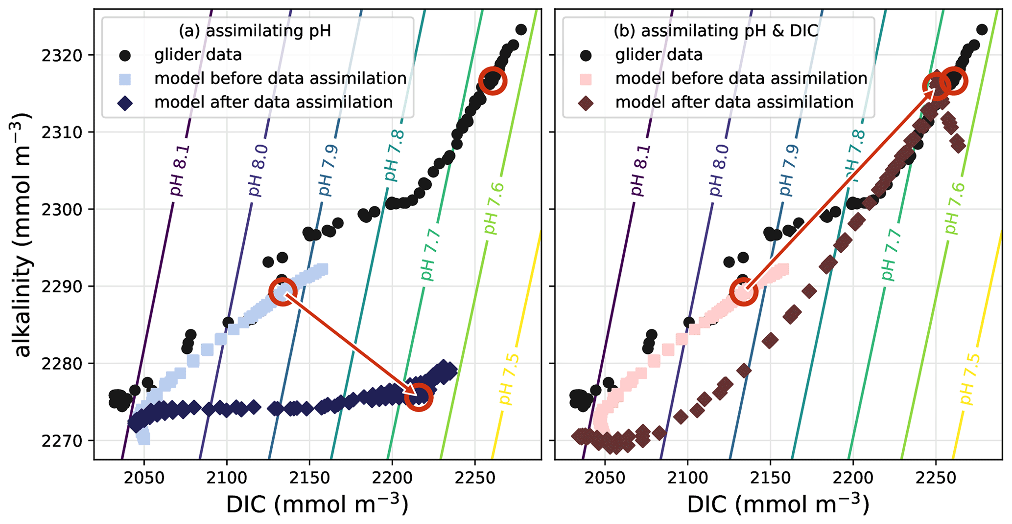
Figure 5Example of a DA application for state estimation of carbonate system properties within a three-dimensional model of the California Current System. The symbols show glider data and model estimates at the measurement times and locations; one specific data point and its associated model estimates are highlighted by red circles. Each data point consists of measured pH alongside estimated alkalinity and DIC values (see Takeshita et al., 2021, for data source and details). In the model, pH is a diagnostic variable and primarily dependent on the model's alkalinity and DIC estimates. (a) When only pH data are assimilated, the model estimates are moved closer to the observed pH values by increments in alkalinity–DIC space that degrade the model's alkalinity estimates. (b) The model state estimates improve considerably by assimilating data for DIC (or alkalinity; not shown) together with the pH observations.
Application of DA for ocean models is typically applied for one of two purposes: (1) to systematically optimize model parameters, e.g., phytoplankton growth and nutrient uptake or rates of background dispersion, and (2) to estimate the ocean state, e.g., distributions of temperature, phytoplankton biomass, alkalinity (see Fennel et al., 2022, for more details on the practical approaches and examples). The first purpose addresses systematic errors and biases in models and is useful when systematically modifying and testing different model formulations, while the second assumes an unbiased model and addresses unresolved stochasticity, e.g., correcting the locations of mesoscale eddies and current meanders. State estimation offers the potential to constrain variability such that OAE-induced perturbations of carbonate system parameters can be documented even if they are smaller than the natural variability in the study region. Joint estimation of physical and biogeochemical properties is common and can yield significant improvements for both types of properties (Yu et al., 2018). Hybrid approaches combining parameter and state estimation have also been proposed (Kitagawa, 1998; Mattern et al., 2012, 2014) but are less widely used.
Successful application of DA critically requires sufficient observations either of the properties that the model parameters to be estimated depend on or of the state variables that are being estimated. The most commonly used observation type in biogeochemical DA applications is satellite-based ocean colour observations (Mattern et al., 2017; Ciavatta et al., 2018; Teruzzi et al., 2018), which are available at a relatively high temporal resolution and cover large areas of the surface ocean. While these observations are useful for informing model estimates of properties directly linked to processes involving phytoplankton, they provide little information on the carbonate system. Dynamical models are able to quantitatively constrain processes that cannot be measured directly by inferring them from observable properties, but only if the observations contain enough relevant information about the processes of interest. Hence, one of the biggest challenges facing the application of DA to models of the marine carbonate system is the sparsity of observations of the marine carbonate system. Observations of pH, pCO2, alkalinity, and DIC used to be limited to moorings and research cruises but have more recently been extended by automated observing systems, such as gliders, BGC-Argo floats, and uncrewed surface vehicles (Bushinski et al., 2019). Although these measurements are becoming more common (Chai et al., 2020), they are still sparse compared to what is typically required for DA applications. In this context, an additional challenge is the problem of underdetermination, i.e., if multiple processes or properties of interest can cause a similar change in an observable property, then observing this property alone may not hold enough information to constrain these processes or properties, and more observations are needed (see Fig. 5 and code examples in Fennel et al., 2022). As new platforms are added to the observing system, DA techniques can help guide their optimal deployment and tailor observational programs to the specific needs of OAE applications (see Sect. 4.3 below). Furthermore, statistical and machine-learning approaches are being developed (e.g., Lohrenz et al., 2018; Bittig et al., 2018) that may help overcome the undersampling of carbonate system properties and could feed directly into DA applications.
There is an important subtlety to the application of data-assimilative models when quantifying net CO2 uptake due to OAE, which is highly relevant for MRV. When the net CO2 uptake is quantified by calculating the difference between two simulations, one with and one without OAE (one of these is realistic, the other counterfactual), it is not appropriate to assimilate biogeochemical observations of properties affected by the alkalinity enhancement. The assimilation of alkalinity-related observations to constrain one of the simulations in the pair would eliminate the ability to make comparisons between the two. However, assimilation of observations that are unaffected by OAE (e.g., temperature, salinity, oxygen, etc.) can be applied to both simulations of the pair. Further research and method development are required to identify the best approaches for leveraging DA in this context.
3.4 Uncertainty analysis
Model results should be paired with sound qualitative and quantitative uncertainty estimates, especially when used for practical decisions. Estimating the uncertainty in model simulations, however, is inherently difficult because typically one is most interested in simulation outputs for which observations are not available (e.g., unobserved or insufficiently observed properties or fluxes in the past, properties and fluxes in the future); hence, standard procedures and metrics for model validation (Sect. 3.2) are not helpful for this aspect. Uncertainty estimates could be based on extensive model parameter and configuration sensitivity studies and comparisons with models that include more realistic representations of uncertain or parameterized processes. Furthermore, since specification of uncertainty is an integral part of DA, DA methodologies provide a useful framework for estimating uncertainty, especially ensemble-based methods.
Any DA application requires uncertainty specification of the observations that are assimilated and can provide uncertainty estimates of the results of the assimilation procedure. Specification of uncertainty in the input data is necessary to inform the DA machinery about how much weight and reach each data point or data type should have in influencing the outcome. The more realistic the uncertainties in the input data, the better the DA outcomes in terms of explanatory or predictive skill. It is important to note that “better” does not mean more precise in this context. Overconfidence in the accuracy of assimilated observations will lead to overfitting and a degradation of predictive skill. In the case of parameter optimization, the output of the assimilation exercise is a set of optimized parameters. The uncertainty in optimal parameters, referred to as a posteriori errors, is determined by a Hessian analysis of the cost function in combination with the uncertainty in the input parameters before optimization, the so-called a priori errors (Thacker, 1989; Fennel et al., 2001). In the case of ensemble-based state estimation, the ensemble spread of the reanalyzed model state provides a spatially and temporally resolved estimate of the uncertainty in the reanalysis (Yu et al., 2018; Hu et al., 2012).
However, an important caveat is that subjectivity enters the uncertainty specification in all of these approaches. For example, in the case of parameter optimization the assumed a priori errors, their probability distributions, and the choice of the cost function are subjective and influence the a posteriori errors (but interestingly the values of the observations themselves do not). In the case of ensemble-based state estimation, the sources of uncertainty inherent in the model simulation have to be specified and simulated by generating variations within a model ensemble. Sources of uncertainty include errors in atmospheric forcing and boundary conditions, model parameters, and structural uncertainty. Uncertainty in forcing and boundary conditions is often represented by perturbing the time of sampling, uncertainty in parameters is represented by sampling from a probability distribution (based on a priori assumptions about the uncertainty in each parameter), and the structural uncertainty is typically represented via brute force inflation factors that amplify ensemble spread. Yu et al. (2018), Li et al. (2016), and Thacker et al. (2012) provide examples where different sources of model uncertainty are accounted for. While the mechanics by which the model ensemble is generated and spreads over time are thus subjective, grossly inappropriate choices will lead to obviously wrong or degraded reanalyses. The success of a DA exercise, which is best judged by an evaluation of whether the predictive power of the model has improved, thus provides a useful reality check on whether the choices for specifying uncertainty were appropriate.
How can the framework for specifying and estimating uncertainty from model ensembles be applied in the context of OAE research? Two different cases should be considered here: (1) model applications where the absolute value of quantities matters for the research question to be addressed and thus the uncertainty in the simulated output and (2) applications where information about the difference between a simulation with and without OAE is of interest and the uncertainty in this difference (e.g., the net CO2 uptake and its uncertainty in the context of MRV). Examples of the first case include studies of the stability of added alkalinity (i.e., simulation of runaway calcium carbonate precipitation) and studies about the exposure of planktonic and benthic communities to high pH. In this case, the ensemble framework described above can be applied with the caveat that the specification of all the relevant sources of uncertainty is by no means trivial and subjective to some degree.
The second case is highly relevant for MRV of OAE, where one is interested in accurately quantifying the increase in seawater DIC due to OAE with well-characterized uncertainty. In this case, one would use two simulations that are based on an identical model set-up with only one difference, namely a source of alkalinity is applied to one (i.e., one of these two simulations is counterfactual or hypothetical; the other would typically be as realistic as possible). It may be tempting and is conceptually straightforward to apply the ensemble framework for each model of the pair and combine the resulting uncertainties via error propagation. However, in practice this would not provide meaningful estimates because there are sources of uncertainty that are unaffected by OAE (e.g., atmospheric forcing), and accounting for them may significantly overestimate uncertainty in the estimated net CO2 uptake. A more appropriate approach would be to construct an ensemble of model pairs that explicitly accounts for uncertainty related to the impacts of alkalinity addition. How to specify and simulate the sources of uncertainty directly resulting from OAE in practice remains an open research question.
In this section, we lay out general objectives for model experimentation in the context of OAE research and provide a short historical view of how these model studies have evolved (Sect. 4.1) followed by specific recommendations for observing system simulation experiments (Sect. 4.2) and model intercomparisons (Sect. 4.3).
4.1 General objectives of model experimentation
General objectives of OAE modelling include (1) gaining a better understanding of the biogeochemistry of OAE, including its effectiveness and side effects; (2) supporting experiments, field trials, or commercial deployments, including through the optimization of observing systems; (3) assessing global carbon-cycle and climate feedbacks; (4) understanding the role that OAE can play in climate mitigation efforts; and (5) supporting monitoring, reporting, and verification activities. At a conceptual level, model approaches for OAE can be classified as belonging to one of two groups: idealized or realistic. Idealized modelling approaches are typically driven by research questions of a fundamental nature and aim to develop or test hypotheses or provide improved process understanding while strongly simplifying a range of potentially complicating factors. They are useful for illustrating cause-and-effect relationships and the range of plausible outcomes given strong assumptions. In contrast, realistic modelling approaches aim to include a broad range of contributing factors as accurately as possible and provide detailed hindcasts or predictions that, if the model has skill, can be used for a range of practical applications. In practice, the dividing line between idealized and realistic models is blurry. Of course, no model will ever simulate all aspects of reality; hence even realistic simulations make many assumptions and are prone to errors from multiple sources. It can be effective to apply idealized and realistic approaches in a complementary manner and iteratively.
It is illustrative to briefly review how modelling for OAE research has developed over the course of the last decade. Much of the early work on OAE used idealized models. Model simulations were designed to investigate whether the theoretical concept of OAE could remove large amounts of CO2 on the global scale. Rather than trying to account for the technical and socio-economic constraints of OAE deployment, the model experiments were designed to investigate what would happen if surface alkalinity were homogeneously increased by massive amounts via a constant addition rate over extremely large regions of the ocean, e.g., in all sea-ice-free waters (Paquay and Zeebe, 2013; Keller et al., 2014; Ilyina et al., 2013; Köhler et al., 2010, 2013). These simulated OAE deployments will never be realized, but the model results suggested that OAE can be viable as a CDR approach. A particular advantage of this idealized approach is that the effect of OAE was easy to detect against internal model variability; i.e., the signal-to-noise ratio is high. The next steps in modelling OAE have remained idealized but have begun to introduce more constraints and better mechanistic or empirically derived components as the experimental OAE date becomes available. Recently, modelling studies tailored to specific regions and modes of application have been conducted to support field trials or commercial deployment (Mongin et al., 2021; Wang et al., 2023). These applications must be as realistic as possible. None of the modelling studies published to date have simulated an actual OAE field trial.
4.2 Recommendations for observing system simulation experiments (OSSEs)
Observing system simulation experiments (OSSEs) use data-assimilative simulations to design new, or modify existing, observing systems such that deployments of observing assets, e.g., floats, gliders, moorings, or surface vehicles, are optimized. General overviews and best practices for OSSEs are provided by Halliwell et al. (2015) and Hoffman and Atlas (2016). Examples of applications to biogeochemical models include Ford (2021), Wang et al. (2020), and Denvil-Sommer et al. (2021). Their goal is to maximize the information gained from a new or modified observing system while keeping the number of required instruments, sensors, or deployments – and thereby cost and effort – low. OSSEs are especially valuable tools in the context of OAE research because the marine carbonate system is still undersampled, observing systems need to be designed and expanded, and new instruments need to be deployed and configured (Boyd et al., 2023).
In practice, this is done with the help of a pair of two different models or model versions, also referred to as twin experiments, as follows. A simulation of one of the models is considered to be the “truth.” This simulation is also referred to as the “nature run”, and synthetic observations are generated by subsampling this nature run. This subsampling can be repeated with different sampling schemes (e.g., different variable types; different numbers of profiles, transects, and/or fixed-location time series; etc.) to represent different configurations of the observing system. Finally, the synthetic observations are assimilated into the other model for which a non-assimilative simulation, the so-called “free run,” is also available. The skill of this data-assimilative simulation, also referred to as the “forecast run,” can be assessed against the free run using independent observations that are also sampled from the nature run. In this way the impact of different sets of observations on the data-assimilative model can be measured and assessed.
While conceptually straightforward, care and consideration are required when setting up OSSEs. For example, the choice of the two model versions making up the twin is important. If the models chosen for the truth and forecast runs are versions of the same model implementation that were generated by perturbing initial, forcing, or boundary conditions in one of them, the method is referred to as the “identical-twin” approach. If two different model types are used, they are “non-identical twins”. The intermediate approach, where the same model type is used but in different configurations (e.g., different physical parameterizations and/or spatial resolution), is referred to as fraternal twin. The identical-twin approach has been more common in oceanic DA applications, although atmospheric OSSEs have shown that it can provide biased impact assessments (Hoffman and Atlas, 2016) typically because the error growth rate between the truth and forecast runs is insufficient. A direct comparison of the non-identical- and identical-twin approach for an ocean circulation model of the Gulf of Mexico has been conducted by Yu et al. (2018). In their assessment of the impacts of the existing observing system (consisting of satellites and Argo floats), the identical-twin approach provided overly optimistic improvements in model skill after assimilation of data from some observing assets (specifically sea surface height and temperature) but undervalued the contribution from temperature and salinity profiles. They concluded that skill assessments and OSSEs using the non-identical-twin approach are more robust. Similar concerns likely apply to OSSEs for biogeochemical properties, but this remains to be studied systematically.
4.3 Recommendations for intercomparisons
Coordinated, multi-model studies, commonly called model intercomparison projects, or MIPs, are a common approach to assessing model uncertainty. They can be used to explore the simulated range of model behaviours; to isolate the strengths and weaknesses of different models in a controlled setting; and to interpret, through idealized experiments, inter-model differences (IPCC, 2013). Carefully designed experiments can also offer a way to distinguish between errors particular to an individual model and those that might be more universal and should become priority targets for model improvement (IPCC, 2013). These studies rely on common agreed-upon protocols for simulating certain processes and writing of diagnostic output to ensure that best practices are followed, and results are comparable (e.g., Griffies et al., 2016). The best-known model intercomparison project is probably the Coupled Model Intercomparison Project (CMIP; Eyring et al., 2016), which is currently finishing up its sixth phase. Within CMIP6, the carbon dioxide removal intercomparison project (CDRMIP; Keller et al., 2018) is the first project to develop a model intercomparison experiment for ocean alkalinity enhancement. This and other MIP examples, including those conducted at smaller regional scales (Wilcox et al., 2023), provide a blueprint for developing coordinated multi-model experiments.
The following key practices have proven useful in previous coordinated multi-model comparisons. Since broad participation is typically desired, the protocol should be straightforward for modelling groups to implement, otherwise few will have the resources to participate. In practice this means avoiding new implementations of complex code or requiring too many or too long simulations. If applicable, forcing data should be centrally prepared and provided to participants in a standardized way that enables easy modification or reformatting, if needed, for use with different models. Using common simulations that modelling groups are likely to have completed already, e.g., climate change scenarios, as control runs and experimental branching points is helpful for minimizing the number of additional required simulations. It is useful to establish common practices that facilitate the production and analysis of the model output, e.g., what should be archived and shared (Juckes et al., 2020) and data standards governing the structure and required metadata for model output (Pascoe et al., 2020). Shared software to standardize model output, such as the Climate Model Output Rewriter (CMOR; https://cmor.llnl.gov/, last access: 15 November 2023) commonly used in CMIP, can be helpful. To maximize the use of model output, it should be made available for public download with digital object identifiers (DOIs). The Earth System Grid Federation (ESGF) is an example of such a system (Petrie et al., 2021). If applicable, preparing and providing quality-controlled observational data sets for model evaluation is useful for facilitating analytical efforts (Waliser et al., 2020). Coordinating the analysis is helpful to avoid duplicative efforts and ensure consistent application of evaluation metrics. Finally, the design of a coordinated multi-model experiment and all its procedures should be well documented in publications or permanently archived protocols. It is advisable to test the multi-model experiment with a small subset of models before inviting a large number of participants. Furthermore, it is worth remembering that the science questions must be appropriate. MIPs require much effort, and not every science question needs a MIP to be answered.
A range of modelling tools and analysis methods are available for OAE research to address questions from microscales to global scales; however, each of these tools and methods has limitations and caveats that model users and users of model-generated outputs need to be aware of. Furthermore, this new field of research poses questions and challenges that current tools were not designed to address, necessitating further development.
A common objective of all modelling approaches described in this article is to simulate the spatiotemporal evolution of carbon chemistry properties in seawater by accounting for the physical, chemical, and biological processes that determine this evolution. Idealized models, which neglect some aspects of reality in the interest of simplicity and clarity of assumptions, have long been used to test basic questions about OAE. As research questions are becoming more focussed on the practical aspects, feasibility, and ecosystem impacts of OAE, more realistic models are increasingly desirable. A skilful realistic model can provide spatial and temporal context for observations, including estimates of properties and fluxes not directly observed. Such models will include parameterizations of the relevant processes for the research objective to be addressed and will be constrained by observations that contain sufficient meaningful information. However, model formulations of several properties and processes relevant to OAE research remain uncertain or highly simplified. For example, presently used model representations of alkalinity in seawater are likely inadequate and may require explicit representation of at least some of the multiple biotic and abiotic sources and sinks of alkalinity; the mechanisms and triggers for spontaneous calcium carbonate precipitation are only beginning to be described and are not yet represented in models; and the impacts of pH perturbations on plankton diversity and trophic interactions remain an active area of study and unaccounted in biogeochemical models. Furthermore, it is difficult to obtain solid constraints on the seawater carbonate system, especially in sufficient spatial and temporal resolution for robust model validation and DA. Theoretically, knowledge of two of the carbonate system parameters allows calculation of the others, but unfortunately pCO2 and pH, the pair most accessible to autonomous measurement, result in high uncertainties.
One inherent challenge to OAE research is the multiscale nature of many of the relevant questions. Different modelling tools are available for different spatial scales. While some research questions may fall neatly within the limited spatial range of a particular model, many do not and require a bridging of scales that could be accomplished via new parameterizations yet to be developed or dynamic coupling of different modelling tools. It is important to emphasize that models have to be tailored to the questions they are meant to address. This means considering what level of model complexity is required and seeking parsimonious representations that are well supported by empirical constraints.
It is important to note that even after thorough validation, any model simulation will be prone to errors and uncertainties due to inaccuracies in model inputs, structural uncertainty due to numerical approximation schemes and insufficient process understanding or representation, and inaccurate model parameters and parameterizations. Deviations between models and reality can be reduced by DA, which is typically applied either to systematically optimize model parameters or to produce optimal estimates of the ocean state. Optimization of model parameters addresses systematic model errors and biases; it is useful for systematic testing of different model formulations during model design. State estimation assumes an unbiased model and addresses unresolved stochasticity, thus leading to model states that are in better agreement with the observed ocean state. However, successful application of DA critically requires sufficient observations. Currently, the biggest impediment to implementing data-assimilative models for OAE research is the sparsity of carbonate system observations. OSSEs, data-assimilative simulations that inform how to place observing assets most effectively, will prove useful in this context. It should also be noted that assimilation of carbonate system parameters is not appropriate when models are applied for MRV.
Uncertainty analysis is a necessary component of any quantitative research and will be an essential deliverable for effective approaches to MRV. Ensemble-based DA methodologies provide a useful framework for estimating uncertainty. Consideration of this framework illustrates that the “law of conservation of difficulty” applies here. Quantitative assumptions about the uncertainty distributions of input data and input parameters and of structural uncertainties inherent in the model are required to obtain an uncertainty estimate of the model output; in other words, difficult assumptions about errors have to be made somewhere. A common approach to assessing model uncertainty is by coordinated, multi-model intercomparison. Such studies can be used to explore the range of simulated behaviours and the strengths and weaknesses of different models, and, by elucidating inter-model differences, they can offer guidance on priority targets for model improvement.
Key recommendations arising from this article are as follows:
-
Idealized models of particle–fluid interaction are recommended to address questions about dissolution and precipitation kinetics at the scale of particles; realistic local-scale models are recommended for addressing questions about near-field processes in the turbulent environment around injection sites; and larger-scale regional or global ocean models are recommended to support observational design for field experiments, to demonstrate possible verification frameworks, and to address questions about global-scale feedbacks on ocean biogeochemistry.
-
When simulating OAE approaches that may generate high oversaturation with respect to carbonate, spontaneous precipitation of carbonates needs to be considered, and appropriate approaches should be developed, e.g., using near-field models to mechanistically represent this process and a meta-model approach to develop parameterizations that are suitable for far-field and larger-scale models.
-
Shortcomings in current-generation models in terms of representing physiological responses of the plankton community to OAE (especially when using crushed-rock feedstocks) need to be recognized, better qualified, and addressed. Empirical research exploring physiological sensitivities should be used to develop prioritizations of key model processes comprising early targets for implementation.
-
The exchange of solutes between the sediments and overlying water influences the seawater carbonate system with DIC from the remineralization of organic matter being returned to overlying water (and alkalinity if this remineralization occurs anaerobically), dissolution of CaCO3 releasing alkalinity, and burial of CaCO3 acting as an alkalinity sink. Accounting for these exchanges between sediments and overlying water and its variability on tidal, seasonal, interannual, and millennial timescales will likely be necessary in regional and global biogeochemical models that aim to simulate alkalinity cycling.
-
River inputs of alkalinity and DIC in regional and global ocean biogeochemical models, including fluxes resulting from land-based CDR applications, should be accurately accounted for. Efforts should be made to improve quantification of riverine fluxes resulting from ongoing field trials and commercial applications and to establish initiatives to effectively track the solute additions from terrestrial alkalinity enhancements.
-
When simulating large-scale deployment of OAE in ocean-only models with prescribed atmospheric CO2, the subtle changes in the atmospheric CO2 inventory resulting from CDR should be accounted for.
-
Models should be tailored to the specific questions they are meant to address while seeking parsimonious representations that are well supported by empirical constraints. For example, for the purpose of MRV it may be appropriate to neglect biological dynamics since the core target is to capture the net air–sea CO2 exchange associated with the OAE-induced surface ocean pCO2 anomaly.
-
Model validation should be an integral part of model implementation and application. For OAE research, validation is a two-step challenge. First, it is necessary to validate unperturbed model baselines to gain confidence that the natural variability is represented appropriately and to quantify model uncertainties. Second, it should be verified that the model accurately represents the perturbations of an alkalinity addition.
-
Since no single model validation metric provides a complete picture of a model's skill, multiple complementary metrics should be used in combination. Furthermore, different points in space and time and a breadth of variable types should be part of any comprehensive validation.
-
Data assimilation, the process of improving the dynamical behaviour of models by statistically combining them with observations, should be employed in order to obtain the most accurate model simulations possible, e.g., to optimize model parameters or to estimate the ocean state. The former addresses systematic errors and biases in models, while the latter assumes an unbiased model and addresses unresolved stochasticity.
-
When applying data-assimilative models for quantification of the OAE-induced net CO2 uptake by calculating the difference between a realistic and a counterfactual simulation, it is not appropriate to assimilate biogeochemical observations of properties affected by the alkalinity enhancement as this would eliminate the ability to make valid comparisons between the two simulations. However, assimilation of observations that are unaffected by OAE can be applied to both simulations of the pair.
-
Successful application of DA critically requires sufficient observations either of the properties that the model parameters to be estimated depend on or of the state variables that are being estimated. Observing system simulation experiments are recommended to design observing strategies tailored to the needs of specific OAE applications.
-
Model results should be paired with sound qualitative and quantitative uncertainty estimates, especially when used for practical decisions. DA methodologies provide a useful framework for estimating uncertainty, especially ensemble-based methods. Coordinated, multi-model studies, commonly called model intercomparison projects, or MIPs, are another common approach to assessing model uncertainty.
The base LES code is available at https://github.com/CliMA/Oceananigans.jl (last access: 15 November 2023; Ramadhan et al., 2020). The ROMS code is available at https://perma.cc/3BJY-U4LE (Haidvogel et al., 2008). The University of Victoria Earth System Climate Model is available at https://perma.cc/8VUY-BHSP (Weaver et al., 2001).
No data sets were used in this article.
KF and MCL conceptualized the article. KF contributed Fig. 4 and drafted Sects. 1, 2.1.2, 2.3, 3.4, and 5. MCL drafted Sects. 2.1.3, 2.1.4, and 3.2. CA drafted Sect. 2.2.3. BC drafted Sect. 3.1. DK contributed Fig. 3 and drafted Sect. 4.1 and 4.3. AL contributed Fig. 2 and content in Sect. 2.1.2. JPM contributed Fig. 5 and drafted Sects. 3.3 and 4.2. RM drafted Sect. 2.1.1 and 2.2.5 together with DBW and JO. AO drafted Sect. 2.2.1 and 2.2.2. JO contributed Fig. 1 and drafted Sect. 2.2.5 with RM. JBP drafted Sect. 2.2.4. KF edited all section drafts and produced a coherent manuscript. All authors contributed to reviewing and editing the complete draft.
Competing interests are declared in a summary for the entire volume at: https://sp.copernicus.org/articles/sp-oae2023-ci-summary.zip.
Publisher’s note: Copernicus Publications remains neutral with regard to jurisdictional claims made in the text, published maps, institutional affiliations, or any other geographical representation in this paper. While Copernicus Publications makes every effort to include appropriate place names, the final responsibility lies with the authors.
We thank the Ocean Acidification and other ocean Changes – Impacts and Solutions (OACIS), an initiative of the Prince Albert II of Monaco Foundation, for its support throughout the project. We extend our gratitude to the Villefranche Oceanographic Laboratory for supporting the meeting of the lead authors in January 2023. Jessica Oberlander's assistance in compiling the bibliography is gratefully acknowledged.
Katja Fennel, Arnaud Laurent, Ruth Musgrave, and Josiane Ostiguy acknowledge funding by NSERC's Discovery and Alliance programs. Katja Fennel, David Keller, Arnaud Laurent, and Andreas Oschlies are supported by the Ocean Alk-Align project funded by Carbon to Sea. Ruth Musgrave is supported by the Canada Research Chairs program. Jann Paul Mattern is supported by the Simons Collaboration on Computational Biogeochemical Modeling of Marine Ecosystems (grant ID: 459949FY22) and the NOAA Ocean Acidification program (grant ID: NA19OAR0170357). Daniel B. Whitt is supported by the NASA Earth Science New Investigator program.
This research has been supported by the ClimateWorks Foundation (grant no. 22-0296) and the Prince Albert II of Monaco Foundation. It has also been supported by NSERC's Discovery and Alliance programs, the Ocean Alk-Align project funded by Carbon to Sea, the Canada Research Chairs program, the Simons Collaboration on Computational Biogeochemical Modeling of Marine Ecosystems (grant no. 459949FY22), the NOAA Ocean Acidification program (grant no. NA19OAR0170357), and the NASA Earth Science New Investigator program.
This paper was edited by Lennart Bach and reviewed by Steve Rackley and two anonymous referees.
Aller, R. C.: Transport and reactions in the bioirrigated zone, in: The Benthic Boundary Layer, edited by: Boudreau, B. P., and Jorgensen, B. B., Oxford University Press, 269–301, ISBN 9780195118810, 2001.
Bach, L. T., Gill, S. J., Rickaby, R. E., Gore, S., and Renforth, P.: CO2 Removal With Enhanced Weathering and Ocean Alkalinity Enhancement: Potential Risks and Co-benefits for Marine Pelagic Ecosystems, Front. Clim., 1, 7, https://doi.org/10.3389/fclim.2019.00007, 2019.
Barrett, P. M., Resing, J. A., Buck, N. J., Freely, R. A., Bullister, J. L., Buck, C. S., and Landing, W. M.: Calcium carbonate dissolution in the upper 1000 m of the eastern North Atlantic, Global Biogeochem. Cy., 28, 386–397, https://doi.org/10.1002/2013GB004619, 2014.
Barton, A. D., Pershing, A. J., Litchman, E., Record, N. R., Edwards, K. F., Kinkel, Z. V., Kiørboe, T., and Ward, B. A.: The biogeography of marine plankton traits, Ecol. Lett., 16, 522–534, https://doi.org/10.1111/ele.12063, 2013.
Bates, N. R. and Merlivat, L.: The influence of short-term wind variability on air-sea CO2 exchange, Geophys. Res. Lett., 28, 3281–3284, https://doi.org/10.1029/2001GL012897, 2001.
Bell, T. G., Landwehr, S., Miller, S. D., de Bruyn, W. J., Callaghan, A. H., Scanlon, B., Ward, B., Yang, M., and Saltzman, E. S.: Estimation of bubble-mediated air–sea gas exchange from concurrent DMS and CO2 transfer velocities at intermediate–high wind speeds, Atmos. Chem. Phys., 17, 9019–9033, https://doi.org/10.5194/acp-17-9019-2017, 2017.
Bittig, H. C., Steinhoff, T., Claustre, H., Fiedler, B., Williams, N. L., Sauzède, R., Körtzinger, A., and Gattuso, J.-P.: An Alternative to Static Climatologies: Robust Estimation of Open Ocean CO2 Variables and Nutrient Concentrations From T, A, and O2 Data using Bayesian Neural Networks, Front. Mar. Sci., 5, 328, https://doi.org/10.3389/fmars.2018.00328, 2018.
Bleninger, T. and Jirka, G. H.: Near- and Far-Field Model Coupling Methodology for Wastewater Discharges, in: Environmental Hydraulics and Sustainable Water Management, edited by: Lee, J. H. W. and Lam, K. M., Taylor & Francis, London, 447–453, https://doi.org/10.1201/b16814, 2004.
Boudreau, B. P. (Eds.): Diagenetic Models and their Implementation: Modelling Transport and Reactions in Aquatic Sciences, Springer, https://doi.org/10.1007/978-3-642-60421-8, 1997.
Boudreau, B. P., Middelburg, J. J., and Meysman, F. J. R.: Carbonate compensation dynamics, Geophys. Res. Lett., 37, L03603, https://doi.org/10.1029/2009GL041847, 2010.
Boudreau, B. P., Middelburg, J. J., and Luo, Y.: The role of calcification in carbonate compensation, Nat. Geosci., 11, 894–900, https://doi.org/10.1038/s41561-018-0259-5, 2018.
Boyd, P. W., Claustre, H., Legendre, L., Gattuso, J.-P., and Le Traon, P.-Y.: Operational monitoring of open-ocean carbon dioxide removal deployments: Detection, attribution, and determination of side effects, in: Frontiers in Ocean Observing: Emerging Technologies for Understanding and Managing a Changing Ocean, edited by: Kappel, E. S., Cullen, V., Costello, M. J., Galgani, L., Gordó-Vilaseca, C., Govindarajan, A., Kouhi, S., Lavin, C., McCartin, L., Müller, J. D., Pirenne, B., Tanhua, T., Zhao, Q., and Zhao, S., Oceanography, 36 (Supplement 1), 2–10, https://doi.org/10.5670/oceanog.2023.s1.2, 2023.
Briggs, E. M., Sandoval, S., Erten, A., Takeshita, Y., Kummel, A. C., and Martz, T. R.: Solid state sensor for simultaneous measurement of total alkalinity and pH of seawater, ACS Sens., 2, 1302–1309, https://doi.org/10.1021/acssensors.7b00305, 2017.
Burdige, D. J.: Preservation of Organic Matter in Marine Sediments: Controls, Mechanisms, and an Imbalance in Sediment Organic Carbon Budgets?, Chem. Rev., 107, 467–485, https://doi.org/10.1021/cr050347q, 2007.
Burt, D. J., Fröb, F., and Ilyina, T.: The sensitivity of the marine carbonate system to regional ocean Alkalinity Enhancement, Front. Clim., 3, 624075, https://doi.org/10.3389/fclim.2021.624075, 2021.
Bushinsky, S. M., Takeshita, Y., and Williams, N. L.: Observing changes in ocean carbonate chemistry: Our autonomous future, Current Climate Change Reports, 5, 207–220, https://doi.org/10.1007/s40641-019-00129-8, 2019.
Carrassi, A., Bocquet, M., Bertino, L., and Evensen, G.: Data assimilation in the geosciences: An overview of methods, issues, and perspectives, WIREs Clim Change, 9, e535, https://doi.org/10.1002/wcc.535, 2018.
Carroll, D., Menemenlis, D., Adkins, J. F., Bowman, K. W., Brix, H., Dutkiewicz, S., Fenty, I., Gierach, M. M., Hill, C., Jahn, O., Landschützer, P., Lauderdale, J. M., Liu, J., Manizza, M., Naviaux, J. D., Rödenbeck, C., Schimel, D. S. Van der Stockem T., and Zhang, H.:The ECCO-Darwin data-assimilative global ocean biogeochemistry model: Estimates of seasonal to multidecadal surface ocean pCO2 and air-sea CO2 flux, J. Adv. Model. Earth Sy., 12, e2019MS001888, https://doi.org/10.1029/2019MS001888, 2020.
Caserini, S., Pagano, D., Campo, F., Abbà, A., De Marco, S., Righi, D., Renforth, P., and Grosso, M.: Potential of maritime transport for ocean liming and atmospheric CO2 removal, Front. Clim., 3, 575900, https://doi.org/10.3389/fclim.2021.575900, 2021.
Ciavatta, S., Brewin, R. J. W., Skákala, J., Polimene, L., de Mora, L., Artioli, Y., and Allen, J. I.: Assimilation of ocean-color plankton functional types to improve marine ecosystem simulations, J. Geophys. Res.-Oceans, 123, 834–854, https://doi.org/10.1002/2017JC013490, 2018.
Chai, F., Johnson, K. S., Claustre, H., Xing, X., Wang, Y., Boss, E., Riser, S., Fennel, K., Schofield, O., and Sutton, A.: Monitoring ocean biogeochemistry with autonomous platforms, Nat. Rev. Earth Environ., 1, 315–326, https://doi.org/10.1038/s43017-020-0053-y, 2020.
Chang, Y. S. and Scotti, A.: Modeling unsteady turbulent flows over ripples: Reynolds-averaged Navier-Stokes equations (RANS) versus large-eddy simulation (LES), J. Geophys. Res.-Oceans, 109, C09012, https://doi.org/10.1029/2003JC002208, 2004.
Chua, E. J., Huettel, M., Fennel, K., and Fulweiler, R. W.: A case for addressing the unresolved role of permeable shelf sediments in ocean denitrification, Limnol. Oceanogr. Lett., 7, 11–25, https://doi.org/10.1002/lol2.10218, 2022.
CMEMS: Global Ocean Physics Analysis and Forecast. E.U. Copernicus Marine Service Information (CMEMS), Marine Data Store (MDS), https://doi.org/10.48670/moi-00016, 2023.
Cossarini, G., Mariotti, L., Feudale, L., Mignot, A., Salon, S., Taillandier, V., Teruzzi, A., and D'Ortenzio, F.: Towards operational 3D-Var assimilation of chlorophyll Biogeochemical-Argo float data into a biogeochemical model of the Mediterranean Sea, Ocean Model., 133, 112–128, https://doi.org/10.1016/j.ocemod.2018.11.005, 2019.
Cullison Gray, S. E., DeGrandpre, M. D., Moore, T. S., Martz, T. R., Friederich, G. E., and Johnson, K. S.: Applications of in situ pH measurements for inorganic carbon calculations, Mar. Chem., 125, 82–90, https://doi.org/10.1016/j.marchem.2011.02.005, 2011.
Denvil-Sommer, A., Gehlen, M., and Vrac, M.: Observation system simulation experiments in the Atlantic Ocean for enhanced surface ocean pCO2 reconstructions, Ocean Sci., 17, 1011–1030, https://doi.org/10.5194/os-17-1011-2021, 2021.
Dickson, A. G. and Riley, J. P.: The estimation of acid dissociation constants in seawater media from potentiometric titrations with strong base. I. The ionic product of water – Kw, Mar. Chem., 7, 89–99, https://doi.org/10.1016/0304-4203(79)90001-X, 1979.
Doney, S. C., Lima, I., Moore, J. K., Lindsay, K., Behrenfeld, M. J., Westberry, T. K., Mahowald, N., Glover, D. M., and Takahashi, T.: Skill metrics for confronting global upper ocean ecosystem-biogeochemistry models against field and remote sensing data, J. Mar. Syst., 76, 95–112, https://doi.org/10.1016/j.jmarsys.2008.05.015, 2009.
Emerson, S. R. and Archer, D.: Calcium carbonate preservation in the ocean, Philos. T. Roy. Soc. S-A., 331, 29–40, https://doi.org/10.1098/rsta.1990.0054, 1990.
European Centre for Medium-Range Weather Forecasts (ECMWF): ECMWF IFS CY41r2 High-Resolution Operational Forecasts, European Centre for Medium-Range Weather Forecasts, 2016, updated monthly, Research Data Archive at the National Center for Atmospheric Research, Computational and Information Systems Laboratory, https://doi.org/10.5065/D68050ZV, 2023.
Eyring, V., Bony, S., Meehl, G. A., Senior, C. A., Stevens, B., Stouffer, R. J., and Taylor, K. E.: Overview of the Coupled Model Intercomparison Project Phase 6 (CMIP6) experimental design and organization, Geosci. Model Dev., 9, 1937–1958, https://doi.org/10.5194/gmd-9-1937-2016, 2016.
Fairall, C. W., Hare, J. E., Edson, J. B., and McGillis, W.: Parameterization and micrometeorological measurement of air-sea gas transfer, Bound.-Lay. Meteorol., 96, 63–106, https://doi.org/10.1023/A:1002662826020, 2000.
Fakhraee, M., Li, Z., Planavsky, N. J., and Reinhard, C. T.: A biogeochemical model of mineral-based ocean alkalinity enhancement: impacts on the biological pump and ocean carbon uptake, Environ. Res. Lett, 18, 044047, https://doi.org/10.1088/1748-9326/acc9d4, 2023.
Farsoiya, P. K., Magdelaine, Q., Antkowiak, A., Popinet, S., and Deike, L.: Direct numerical simulations of bubble-mediated gas transfer and dissolution in quiescent and turbulent flows, J. Fluid Mech., 954, A29, https://doi.org/10.1017/jfm.2022.994, 2023.
Fassbender, A. J. Sabine, C. L., Lawrence-Slavas, N., De Carlo, E. H., Meinig, C., and Maenner Jones, S.: Robust sensor for extended autonomous measurements of surface ocean dissolved inorganic carbon, Environ. Sci. Technol., 49, 3628–3635, https://doi.org/10.1021/es5047183, 2015.
Feng, E. Y., Koeve, W., Keller, D. P., and Oschlies, A.: Model-Based Assessment of the CO2 Sequestration Potential of Coastal Ocean Alkalization, Earths Future, 5, 1252–1266, https://doi.org/10.1002/2017EF000659, 2017.
Fennel, K., Losch, M., Schröter, J., and Wenzel, M.: Testing a marine ecosystem model: sensitivity analysis and parameter optimization, J. Marine Syst., 28, 45–63, https://doi.org/10.1016/S0924-7963(00)00083-X, 2001.
Fennel, K., Wilkin, J., Previdi, M., and Najjar, R.: Denitrification effects on air-sea CO2 flux in the coastal ocean: Simulations for the Northwest North Atlantic, Geophys. Res. Lett., 35, L24608, https://doi.org/10.1029/2008GL036147, 2008.
Fennel, K., Gehlen, M., Brasseur, P., Brown, C. W., Ciavatta, S., Cossarini, G., Crise, A., Edwards, C. A., Ford, D., Friedrichs, M. A. M., Gregoire, M., Jones, E., Kim, H-C., Lamouroux, J., Murtugudde, R., Perruche, C., and the GODAE OceanView Marine Ecosystem Analysis and Prediction Task Team: Advancing Marine Biogeochemical and Ecosystem Reanalyses and Forecasts as Tools for Monitoring and Managing Ecosystem Health, Front. Mar. Sci., 6, 89, https://doi.org/10.3389/fmars.2019.00089, 2019.
Fennel, K., Mattern, J. P., Doney, S., Bopp, L., Moore, A., Wang, B., and Yu, L.: Ocean biogeochemical modelling, Nat. Rev. Methods Primers, 2, 76, https://doi.org/10.1038/s43586-022-00154-2, 2022.
Ferderer, A., Chase, Z., Kennedy, F., Schulz, K. G., and Bach, L. T.: Assessing the influence of ocean alkalinity enhancement on a coastal phytoplankton community, Biogeosciences, 19, 5375–5399, https://doi.org/10.5194/bg-19-5375-2022, 2022.
Ford, D.: Assimilating synthetic Biogeochemical-Argo and ocean colour observations into a global ocean model to inform observing system design, Biogeosciences, 18, 509–534, https://doi.org/10.5194/bg-18-509-2021, 2021.
Fornari, W., Picano, F., Sardinia, G., and Brandt, L.: Reduced particle settling speed in turbulence, J. Fluid Mech., 808, 153–167, https://doi.org/10.1017/jfm.2016.648, 2016.
Foteinis, S., Campbell, J. S., and Renforth, P.: Life cycle assessment of coastal enhanced weathering for carbon dioxide removal from air, Environ. Sci. Technol., 57, 6169–6178, https://doi.org/10.1021/acs.est.2c08633, 2023.
Fry, C. H., Tyrrell, T., Hain, M. P., Bates, N. R., and Achterberg, E. P.: Analysis of global surface ocean alkalinity to determine controlling processes, Mar. Chem., 174, 46–57, https://doi.org/10.1016/j.marchem.2015.05.003, 2015.
Fuhr, M., Geilert, S., Schmidt, M., Liebetrau, V., Vogt, C., Ledwig, B., and Wallmann, K.: Kinetics of olivine weathering in seawater: an experimental study, Front. Clim., 4, 831587, https://doi.org/10.3389/fclim.2022.831587, 2022.
Gehlen, M., Bopp, L., and Aumont, O.: Short-term dissolution response of pelagic carbonate sediments to the invasion of anthropogenic CO2: A model study, Geochem. Geophy. Geosy., 9, Q02012, https://doi.org/10.1029/2007GC001756, 2008.
Gent, P. R. and McWilliams, J. C.: Isopycnal Mixing in Ocean Circulation Models, J. Phys. Oceanogr., 20, 150–155, https://doi.org/10.1175/1520-0485(1990)020<0150:IMIOCM>2.0.CO;2, 1990.
Gentile, E., Tarantola, F., Lockley, A., Vivian, C., and Caserini, S.: Use of aircraft in ocean alkalinity enhancement, Sci. Total Environ., 822, 153484, https://doi.org/10.1016/j.scitotenv.2022.153484, 2022.
Golshan, R., Tejada-Martínez, A. E., Juha, M. J., and Bazilevs, Y.: LES and RANS simulation of wind-and wave-forced oceanic turbulent boundary layers in shallow water with wall modeling, Comput. Fluids, 145, 96–108, https://doi.org/10.1016/j.compfluid.2016.05.016, 2017.
Griffies, S. M., Danabasoglu, G., Durack, P. J., Adcroft, A. J., Balaji, V., Böning, C. W., Chassignet, E. P., Curchitser, E., Deshayes, J., Drange, H., Fox-Kemper, B., Gleckler, P. J., Gregory, J. M., Haak, H., Hallberg, R. W., Heimbach, P., Hewitt, H. T., Holland, D. M., Ilyina, T., Jungclaus, J. H., Komuro, Y., Krasting, J. P., Large, W. G., Marsland, S. J., Masina, S., McDougall, T. J., Nurser, A. J. G., Orr, J. C., Pirani, A., Qiao, F., Stouffer, R. J., Taylor, K. E., Treguier, A. M., Tsujino, H., Uotila, P., Valdivieso, M., Wang, Q., Winton, M., and Yeager, S. G.: OMIP contribution to CMIP6: experimental and diagnostic protocol for the physical component of the Ocean Model Intercomparison Project, Geosci. Model Dev., 9, 3231–3296, https://doi.org/10.5194/gmd-9-3231-2016, 2016.
Grigoratou, M., Monteiro, F. M., Wilson, J. D., Ridgwell, A., and Schmidt, D. N.: Exploring the impact of climate change on the global distribution of non-spinose planktonic foraminifera using a trait-based ecosystem model, Glob. Change Biol., 28, 1063–1076, https://doi.org/10.1111/gcb.15964, 2022.
Guo, J. A., Strzepek, R., Willis, A., Ferderer, A., and Bach, L. T.: Investigating the effect of nickel concentration on phytoplankton growth to assess potential side-effects of ocean alkalinity enhancement, Biogeosciences, 19, 3683–3697, https://doi.org/10.5194/bg-19-3683-2022, 2022.
Haidvogel, D. B., Arango, H., Budgell, W. P., Cornuelle, B. D., Curchitser, E., Lorenzo, E. D., Fennel, K., Geyer, W. R., Hermann, A. J., Lanerolle, L., Levin, J., McWilliams, J. C., Miller, A. J., Moore, A. M., Powell, T. M., Shchepetkin, A. F., Sherwood, C. R., Signell, R. P., Warner, J. C., and Wilkin, J.: Ocean forecasting in terrain-following coordinates: Formulation and skill assessment of the Regional Ocean Modeling System, J. Comput. Phys., 227, 3595–3624, https://doi.org/10.1016/j.jcp.2007.06.016, 2008 (code available at: https://perma.cc/3BJY-U4LE, last access: 15 November 2023).
Hain, M. P., Sigman, D. M., Higgins, J. A., and Haug, G. H.: The effects of secular calcium and magnesium concentration changes on the thermodynamics of seawater acid/base chemistry: Implications for Eocene and Cretaceous ocean carbon chemistry and buffering, Global Biogeochem. Cy., 29, 517–533, https://doi.org/10.1002/2014GB004986, 2015.
Halliwell, G. R., Kourafalou, V., Le Hénaff, M., Shay, L. K., and Atlas, R.: OSSE impact analysis of airborne ocean surveys for improving upper-ocean dynamical and thermodynamical forecasts in the Gulf of Mexico, Prog. Oceanogr., 130, 32–46, https://doi.org/10.1016/j.pocean.2014.09.004, 2015.
Hartmann, J., Suitner, N., Lim, C., Schneider, J., Marín-Samper, L., Arístegui, J., Renforth, P., Taucher, J., and Riebesell, U.: Stability of alkalinity in ocean alkalinity enhancement (OAE) approaches – consequences for durability of CO2 storage, Biogeosciences, 20, 781–802, https://doi.org/10.5194/bg-20-781-2023, 2023.
Harvey, L. D. D.: Mitigating the atmospheric CO2 increase and ocean acidification by adding limestone powder to upwelling regions, J. Geophys. Res., 113, C04028, https://doi.org/10.1029/2007JC004373, 2008.
He, J. and Tyka, M. D.: Limits and CO2 equilibration of near-coast alkalinity enhancement, Biogeosciences, 20, 27–43, https://doi.org/10.5194/bg-20-27-2023, 2023.
Heuzé, C.: Antarctic Bottom Water and North Atlantic Deep Water in CMIP6 models, Ocean Sci., 17, 59–90, https://doi.org/10.5194/os-17-59-2021, 2021.
Hinrichs, C., Köhler, P., Völker, C., and Hauck, J.: Alkalinity biases in CMIP6 Earth system models and implications for simulated CO2 drawdown via artificial alkalinity enhancement, Biogeosciences, 20, 3717–3735, https://doi.org/10.5194/bg-20-3717-2023, 2023.
Ho, D. T., Bopp, L., Palter, J. B., Long, M. C., Boyd, P. W., Neukermans, G., and Bach, L. T.: Monitoring, reporting, and verification for ocean alkalinity enhancement, in: Guide to Best Practices in Ocean Alkalinity Enhancement Research, edited by: Oschlies, A., Stevenson, A., Bach, L. T., Fennel, K., Rickaby, R. E. M., Satterfield, T., Webb, R., and Gattuso, J.-P., Copernicus Publications, State Planet, 2-oae2023, 12, https://doi.org/10.5194/sp-2-oae2023-12-2023, 2023.
Hoffman, R. N. and Atlas, R.: Future observing system simulation experiments, B. Am. Meteorol. Soc., 97, 1601–1616, https://doi.org/10.1175/BAMS-D-15-00200.1, 2016.
House, K. Z., House, C. H., Schrag, D. P., and Aziz, M. J.: Electrochemical acceleration of chemical weathering for carbon capture and sequestration, Enrgy. Proced., 1, 4953–4960, https://doi.org/10.1016/j.egypro.2009.02.327, 2009.
Hu, J., Fennel, K., Mattern, J. P., and Wilkin, J.: Data assimilation with a local Ensemble Kalman Filter applied to a three-dimensional biological model of the Middle Atlantic Bight, J. Marine Syst., 94, 145–156, 2012.
Huettel, M., Berg, P., and Kostka, J. E.: Benthic exchange and biogeochemical cycling in permeable sediments, Ann. Rev. Mar. Sci., 6, 23–51, https://doi.org/10.1146/annurev-marine-051413-012706, 2014.
Ilyina, T., Wolf-Gladrow, D., Munhoven, G., and Heinze, C.: Assessing the potential of calcium-based artificial ocean alkalinization to mitigate rising atmospheric CO2 and ocean acidification, Geophys. Res. Lett., 40, 5909–5914, https://doi.org/10.1002/2013GL057981, 2013.
IPCC: Climate Change 2013: The Physical Science Basis, Contribution of Working Group I to the Fifth Assessment Report of the Intergovernmental Panel on Climate Change, edited by: Stocker, T. F., Qin, D., Plattner, G.-K., Tignor, M., Allen, S. K., Boschung, J., Nauels, A., Xia, Y., Bex, V., Midgley, P. M., Cambridge University Press, 1585 pp., ISBN 978-92-9169-138-8, 2013.
Jahnke, R. A.: Global synthesis, in: Carbon and nutrient fluxes in continental margins: A global synthesis, edited by: Liu, K.-K., Atkinson, L., Quiñones, R., and Talaue-McManus, L., Springer, Berlin, Heidelberg, Germany, 597–615, https://doi.org/10.1007/978-3-540-92735-8, 2010.
Jirka, G. H., Doneker, R. L., and Hinton, S. W.: User's manual for CORMIX: A hydrodynamic mixing zone model and decision support system for pollutant discharges into surface waters, U. S. Environmental Protection Agency, Washington, D.C., https://www.epa.gov/sites/default/files/2015-10/documents/cormix-users_0.pdf (last access: 15 November 2023), 1996.
Juckes, M., Taylor, K. E., Durack, P. J., Lawrence, B., Mizielinski, M. S., Pamment, A., Peterschmitt, J.-Y., Rixen, M., and Sénési, S.: The CMIP6 Data Request (DREQ, version 01.00.31), Geosci. Model Dev., 13, 201–224, https://doi.org/10.5194/gmd-13-201-2020, 2020.
Keller, D. P., Oschlies, A., and Eby, M.: A new marine ecosystem model for the University of Victoria Earth System Climate Model, Geosci. Model Dev., 5, 1195–1220, https://doi.org/10.5194/gmd-5-1195-2012, 2012.
Keller, D. P., Feng, E. Y., and Oschlies, A.: Potential climate engineering effectiveness and side effects during a high carbon dioxide-emission scenario, Nat. Commun., 5, 3304, https://doi.org/10.1038/ncomms4304, 2014.
Keller, D. P., Lenton, A., Scott, V., Vaughan, N. E., Bauer, N., Ji, D., Jones, C. D., Kravitz, B., Muri, H., and Zickfeld, K.: The Carbon Dioxide Removal Model Intercomparison Project (CDRMIP): rationale and experimental protocol for CMIP6, Geosci. Model Dev., 11, 1133–1160, https://doi.org/10.5194/gmd-11-1133-2018, 2018.
Kitagawa, G.: A self-organizing state-space model. J. Am. Stat. Assoc., 93, 1203–1215, https://doi.org/10.2307/2669862, 1998.
Ko, Y. H., Lee, K., Eom, K. H., and Han, I.-S.: Organic alkalinity produced by phytoplankton and its effect on the computation of ocean carbon parameters, Limnol. Oceanogr., 61, 1462–1471, https://doi.org/10.1002/lno.10309, 2016.
Koeve, W. and Oschlies, A.: Potential impact of DOM accumulation on fCO2 and carbonate ion computations in ocean acidification experiments, Biogeosciences, 9, 3787–3798, https://doi.org/10.5194/bg-9-3787-2012, 2012.
Köhler, P., Hartmann, J., and Wolf-Gladrow, D. A.: Geoengineering potential of artificially enhanced silicate weathering of olivine, P. Natl. Acad. Sci. USA, 107, 20228–20233, https://doi.org/10.1073/pnas.1000545107, 2010.
Köhler, P., Abrams, J. F., Völker, C., Hauck, J., and Wolf-Gladrow, D. A.: Geoengineering impact of open ocean dissolution of olivine on atmospheric CO2, surface ocean pH and marine biology, Environ. Res. Lett., 8, 014009, https://doi.org/10.1088/1748-9326/8/1/014009, 2013.
Krumhardt, K. M., Lovenduski, N. S., Iglesias-Rodriguez, M. D., and Lkeypas, J. A.: Coccolithophore growth and calcification in a changing ocean, Prog. Oceanogr., 159, 276–295, https://doi.org/10.1016/j.pocean.2017.10.007, 2017.
Laurent, A., Fennel, K., Wilson, R., Lehrter, J., and Devereux, R.: Parameterization of biogeochemical sediment–water fluxes using in situ measurements and a diagenetic model, Biogeosciences, 13, 77–94, https://doi.org/10.5194/bg-13-77-2016, 2016.
Laurent, A., Fennel, K., and Kuhn, A.: An observation-based evaluation and ranking of historical Earth system model simulations in the northwest North Atlantic Ocean, Biogeosciences, 18, 1803–1822, https://doi.org/10.5194/bg-18-1803-2021, 2021.
Laurent, A., Wang, B., Pei, A., Ohashi, K., Sheng, J., Garcia Larez, E., Fradette, C., Rakshit, S., Atamanchuk, D., Azetsu-Scott, K., Algar, C., Wallace, D., Burt, W., and Fennel, K.: A high-resolution nested model to study the effects of alkalinity additions in a mid-latitude coastal fjord, presented at the Ocean Sciences Meeting 2024, 18–23 February 2024, New Orleans, USA, AGU, Abstract number: 1486172, 2024.
Lellouche, J.-M., Greiner, E., Bourdallé-Badie, R., Garric, G., Melet, A., Drévillon, M., Bricaud, C., Hamon, M., Le Galloudec, O., Regnier, C., Candela, T., Testut. C.-E., Gasparin, F., Ruggiero, G., Benkiran, M., Drillet, Y., and Le Traon, P.-Y.: The Copernicus Global ∘ Oceanic and Sea Ice GLORYS12 Reanalysis, Front. Earth Sci., 9, 698876, https://doi.org/10.3389/feart.2021.698876, 2021.
Lewis, E. R. and Wallace, D. W. R.: Program developed for CO2 system calculations, Environmental System Science Data Infrastructure for a Virtual Ecosystem (ESS-DIVE), United States, US Lawrence Berkely National Lab, https://doi.org/10.15485/1464255, 1998.
Li, G., Iskandarani, M., Le Hénaff, M., Winokur, J., Le Maître, O. P., and Knio, O. M.: Quantifying initial and wind forcing uncertainties in the Gulf of Mexico, Computat. Geosci., 20, 1133–1153, https://doi.org/10.1007/s10596-016-9581-4, 2016.
Liang, J.-H., McWilliams, J. C., Sullivan, P. P., and Basckek, B.: Modeling bubbles and dissolved gases in the ocean, J. Geophys. Res.-Oceans, 116, C03015, https://doi.org/10.1029/2010JC006579, 2011.
Liang, J.-H., Deutsch, C., McWilliams, J. C., Baschek, B., Sullivan, P. P., and Chiba, D.: Parameterizing bubble-mediated air-sea gas exchange and its effect on ocean ventilation, Global Biogeochem. Cy., 27, 894–905, https://doi.org/10.1002/gbc.20080, 2013.
Lohrenz, S. E., Cai, W.-J., Chakraborty, S., Huang, W.-J., Guo, X., He, R., Xue, Z., Fennel, K., Howden, S., and Tian, H.: Satellite estimation of coastal pCO2 and air-sea flux of carbon dioxide in the northern Gulf of Mexico, Remote Sens. Environ., 207, 71–83, https://doi.org/10.1016/j.rse.2017.12.039, 2018.
Long, J. S., Hu, C., Robbins, L. L., Byrne, R. H., Paul, J. H., and Wolny, J. L.: Optical and biochemical properties of a southwest Florida whiting event, Estuar. Coast. Shelf S., 196, 258–268, https://doi.org/10.1016/j.ecss.2017.07.017, 2017.
Long, M. C., Moore, J. K., Lindsay, K., Levy, M., Doney, S. C., Luo, J. Y., Krumhardt, K. M., Letscher, R. T., Grover, M., and Sylvester, Z. T.: Simulations with the marine biogeochemistry library (MARBL), J. Adv. Model. Earth Syst., 13, e2021MS002647, https://doi.org/10.1029/2021ms002647, 2021.
Mattern, J. P., Fennel, K., and Dowd, M.: Estimating time-dependent parameters for a biological ocean model using an emulator approach, J. Mar. Syst., 96–97, 32–47, https://doi.org/10.1016/j.jmarsys.2012.01.015, 2012.
Mattern, J. P., Fennel, K., and Dowd, M.: Periodic time-dependent parameters improving forecasting abilities of biological ocean models, Geophys. Res. Lett., 41, 6848–6854, https://doi.org/10.1002/2014GL061178, 2014.
Mattern, J. P., Song, H., Edwards, C. A., Moore, A. M., and Fiechter, J.: Data assimilation of physical and chlorophyll observations in the California Current System using two biogeochemical models, Ocean Model., 109, 55–71, https://doi.org/10.1016/j.ocemod.2016.12.002, 2017.
Maurer, T. L., Plant, J. N., and Johnson, K. S.: Delayed-Mode Quality Control of Oxygen, Nitrate, and pH Data on SOCCOM Biogeochemical Profiling Floats, Front. Mar. Sci., 8, 683207, https://doi.org/10.3389/fmars.2021.683207, 2021.
McLaughlin, K., Weisberg, S. B., Dickson, A. G., Hofmann, G., Newton, J. A., Aseltine-Neilson, D., Barton, A., Cudd, S., Feely, R. A., Jefferds, I. W., Jewett, E. B., King, T., Langdon, C. J., McAfee, S., Pleschner-Steele, D., and Steele, B.: Core principles of the California current acidification network: Linking chemistry, physics, and ecological effects, Oceanography, 28, 160–169, http://www.jstor.org/stable/24861878 (last access: 15 November 2023), 2015.
Mengis, N., Keller, D. P., MacDougall, A. H., Eby, M., Wright, N., Meissner, K. J., Oschlies, A., Schmittner, A., MacIsaac, A. J., Matthews, H. D., and Zickfeld, K.: Evaluation of the University of Victoria Earth System Climate Model version 2.10 (UVic ESCM 2.10), Geosci. Model Dev., 13, 4183–4204, https://doi.org/10.5194/gmd-13-4183-2020, 2020.
Mensa, J. A., Özgökmen, T. M., Poje, A. C., and Imberger, J.: Material transport in a convective surface mixed layer under weak wind forcing, Ocean Model., 96, 226–242, https://doi.org/10.1016/j.ocemod.2015.10.006, 2015.
Meysman, F. J. R. and Montserrat, F.: Negative CO2 emissions via enhanced silicate weathering in coastal environments, Biol. Lett., 13, 20160905, https://doi.org/10.1098/rsbl.2016.0905, 2017.
Meysman, F. J. R., Middelburg, J. J., and Heip, C. H. R.: Bioturbation: a fresh look at Darwin's last idea, Trends Ecol. Evol., 21, 688–695, https://doi.org/10.1016/j.tree.2006.08.002, 2006.
Middelburg, J. J., Soetaert, K., and Hagens, M.: Ocean Alkalinity, Buffering and Biogeochemical Processes, Rev. Geophys., 58, e2019RG000681, https://doi.org/10.1029/2019RG000681, 2020.
Millero, F. J.: The Marine Inorganic Carbon Cycle, Chem. Rev., 107, 308–341, https://doi.org/10.1021/cr0503557, 2007.
Mongin, M., Baird, M. E., Tilbrook, B., Matear, R. J., Lenton, A., Herzfeld, M., Wild-Allen, K., Skerratt, J., Margvelashvili, N., Robson, B. J., Duarte, C. M., Gustafsson, M. S. M., Ralph, P. J., and Steven, A. D. L.: The exposure of the Great Barrier Reef to ocean acidification, Nat. Commun., 7, 10732, https://doi.org/10.1038/ncomms10732, 2016.
Mongin, M., Baird, M. E., Lenton, A., Neill, C., and Akl, J.: Reversing ocean acidification along the Great Barrier Reef using alkalinity injection, Environ. Res. Lett., 16, 064068, https://doi.org/10.1088/1748-9326/ac002d, 2021.
Montserrat, F., Renforth, P., Hartmann, J., Leermakers, M., Knops, P., and Meysman, F. J. R.: Olivine dissolution in seawater: Implications for CO2 sequestration through enhanced weathering in coastal environments, Environ. Sci. Technol., 51, 3960–3972, https://doi.org/10.1021/acs.est.6b05942, 2017.
Moras, C. A., Bach, L. T., Cyronak, T., Joannes-Boyau, R., and Schulz, K. G.: Ocean alkalinity enhancement – avoiding runaway CaCO3 precipitation during quick and hydrated lime dissolution, Biogeosciences, 19, 3537–3557, https://doi.org/10.5194/bg-19-3537-2022, 2022.
Moriarty, J. M., Harris, C. K., Fennel, K., Friedrichs, M. A. M., Xu, K., and Rabouille, C.: The roles of resuspension, diffusion and biogeochemical processes on oxygen dynamics offshore of the Rhône River, France: a numerical modeling study, Biogeosciences, 14, 1919–1946, https://doi.org/10.5194/bg-14-1919-2017, 2017.
Moriarty, J. M., Harris, C. K., Friedrichs, M. A. M., Fennel, K., and Xu, K.: Impact of seabed resuspension on oxygen and nitrogen dynamics in the northern Gulf of Mexico: A numerical modeling study, J. Geophys. Res-Oceans, 123, 7237–7263, https://doi.org/10.1029/2018JC013950, 2018.
Morse, J. W., Mucci, A., and Millero, F. J.: The solubility of calcite and aragonite in seawater of 35 %. Salinity at 25 ∘C and atmospheric pressure, Geochim. Cosmochim. Ac., 44, 85–94, https://doi.org/10.1016/0016-7037(80)90178-7, 1980.
Mu, L., Palter, J. B., and Wang, H.: Considerations for hypothetical carbon dioxide removal via alkalinity addition in the Amazon River watershed, Biogeosciences, 20, 1963–1977, https://doi.org/10.5194/bg-20-1963-2023, 2023.
Naveira Garabato, A. C., MacGilchrist, G. A., Brown, P. J., Evans, D. G., Meijers, A. J. S., and Zika, J. D.: High-latitude ocean ventilation and its role in Earth's climate transitions, Philos. T. Roy. Soc. A, 375, 20160324, https://doi.org/10.1098/rsta.2016.0324, 2017.
Negrete-García, G., Luo, J. Y., Long, M. C., Lindsay, K., Levy, M., and Barton, A. D.: Plankton energy flows using a global size-structured and trait-based model, Prog. Oceanogr., 209, 102898, https://doi.org/10.1016/j.pocean.2022.102898, 2022.
Oschlies, A.: Impact of atmospheric and terrestrial CO2 feedbacks on fertilization-induced marine carbon uptake, Biogeosciences, 6, 1603–1613, https://doi.org/10.5194/bg-6-1603-2009, 2009.
Paquay, F. S. and Zeebe, R. E.: Assessing possible consequences of ocean liming on ocean pH, atmospheric CO2 concentration and associated costs, Int. J. Green. Gas Con., 17, 183–188, https://doi.org/10.1016/j.ijggc.2013.05.005, 2013.
Pascoe, C., Lawrence, B. N., Guilyardi, E., Juckes, M., and Taylor, K. E.: Documenting numerical experiments in support of the Coupled Model Intercomparison Project Phase 6 (CMIP6), Geosci. Model Dev., 13, 2149–2167, https://doi.org/10.5194/gmd-13-2149-2020, 2020.
Paul, A. J. and Bach, L. T.: Universal response pattern of phytoplankton growth rates to increase CO2, New Phytol., 228, 1710–1716, https://doi.org/10.1111/nph.16806, 2020.
Paulmier, A., Kriest, I., and Oschlies, A.: Stoichiometries of remineralisation and denitrification in global biogeochemical ocean models, Biogeosciences, 6, 923–935, https://doi.org/10.5194/bg-6-923-2009, 2009.
Petrie, R., Denvil, S., Ames, S., Levavasseur, G., Fiore, S., Allen, C., Antonio, F., Berger, K., Bretonnière, P.-A., Cinquini, L., Dart, E., Dwarakanath, P., Druken, K., Evans, B., Franchistéguy, L., Gardoll, S., Gerbier, E., Greenslade, M., Hassell, D., Iwi, A., Juckes, M., Kindermann, S., Lacinski, L., Mirto, M., Nasser, A. B., Nassisi, P., Nienhouse, E., Nikonov, S., Nuzzo, A., Richards, C., Ridzwan, S., Rixen, M., Serradell, K., Snow, K., Stephens, A., Stockhause, M., Vahlenkamp, H., and Wagner, R.: Coordinating an operational data distribution network for CMIP6 data, Geosci. Model Dev., 14, 629–644, https://doi.org/10.5194/gmd-14-629-2021, 2021.
Raimondi, L., Matthews, J. B. R., Atamanchuk, D., Azetsu-Scott, K., and Wallace, D. W. R.: The internal consistency of the marine carbon dioxide system for high latitude shipboard and in situ monitoring, Mar. Chem., 213, 49–70, https://doi.org/10.1016/j.marchem.2019.03.001, 2019.
Ramadhan, A., Wagner, G., Hill, C., Campin, J.-M., Churavy, V., Besard, T., Souza, A., Edelman, A., Ferrari, R., and Marshall, J.: Oceananigans.jl: Fast and friendly geophysical fluid dynamics in GPUs, J. Open Source Softw., 5, 2018, https://doi.org/10.21105/joss.02018, 2020 (code available at: https://github.com/CliMA/Oceananigans.jl, last access: 15 November 2023).
Rau, G. H., McLeod, E. L., and Hoegh-Guldberg, O.: The need for new ocean conservation strategies in a high-carbon dioxide world, Nat. Clim. Change, 2, 720–724, https://doi.org/10.1038/nclimate1555, 2012.
Renforth, P. and Henderson, G.: Assessing ocean alkalinity for carbon sequestration, Rev. Geophys., 55, 636–674, https://doi.org/10.1002/2016RG000533, 2017.
Riebesell, U., Wold-Gladrow, D. A., and Smetacek, V.: Carbon dioxide limitation of marine phytoplankton growth rates, Nature, 361, 249–251, https://doi.org/10.1038/361249a0, 1993.
Ringham, M.: High resolution, in-situ studies of seawater carbonate chemistry and carbon cycling in costal systems using CHANnelized Opticals System II, PhD thesis, Massachusetts Institute of Technology, 127 pp., https://hdl.handle.net/1721.1/144860, 2022.
Rothstein, L. M., Cullen, J. J., Abbott, M., Chassignet, E. P., Denman, K., Doney, S. C., Ducklow, H., Fennel, K., Follows, M., Haidvogel, D., Hofmann, E., Karl, D. M., Kindle, J., Lima, I., Maltrud, M., McClain, C., McGillicuddy, D., Olascoaga, M. J., Spitz, Y., Wiggert, J., and Woder, J.: Modeling Ocean Ecosystems: The PARADIGM Program, Oceanography, 19, 22–51, https://doi.org/10.5670/oceanog.2006.89, 2015.
Rutherford, K., Fennel, K., Atamanchuk, D., Wallace, D., and Thomas, H.: A modelling study of temporal and spatial pCO2 variability on the biologically active and temperature-dominated Scotian Shelf, Biogeosciences, 18, 6271–6286, https://doi.org/10.5194/bg-18-6271-2021, 2021.
Sarmiento, J. L. and Gruber, N.: Ocean Biogeochemical Dynamics, Princeton University Press, https://doi.org/10.2307/j.ctt3fgxqx, 2006.
Sauerland, V., Kriest, I., Oschlies, A., and Srivastav, A.: Multiobjective calibration of a global biogeochemical ocean model against nutrients, oxygen, and oxygen minimum zones, J. Adv. Model. Earth Sy., 11, 1285–1308, https://doi.org/10.1029/2018MS001510, 2019.
Schartau, M., Wallhead, P., Hemmings, J., Löptien, U., Kriest, I., Krishna, S., Ward, B. A., Slawig, T., and Oschlies, A.: Reviews and syntheses: parameter identification in marine planktonic ecosystem modelling, Biogeosciences, 14, 1647–1701, https://doi.org/10.5194/bg-14-1647-2017, 2017.
Schmittner, A., Oschlies, A., Matthews, H. D., and Galbraith, E. D.: Future changes in climate, ocean circulation, ecosystems, and biogeochemical cycling simulated for a business-as-usual CO2 emission scenario until 4000 AD, Global Biogeochem. Cy., 22, GB1013, https://doi.org/10.1029/2007GB002953, 2008.
Schulz, K. G., Bach, L. T., and Dickson, A. G.: Seawater carbonate chemistry considerations for ocean alkalinity enhancement research: theory, measurements, and calculations, in: Guide to Best Practices in Ocean Alkalinity Enhancement Research, edited by: Oschlies, A., Stevenson, A., Bach, L. T., Fennel, K., Rickaby, R. E. M., Satterfield, T., Webb, R., and Gattuso, J.-P., Copernicus Publications, State Planet, 2-oae2023, 2, https://doi.org/10.5194/sp-2-oae2023-2-2023, 2023.
Seitzinger, S. P., Harrison, J. A., Böhlke, J. K., Bouwman, A. F., Lowrance, R.,. Tobias, C., and Van Drecht, G.: Denitrification across landscapes and waterscapes: A synthesis, Ecol. Appl., 16, 2064–2090, https://doi.org/10.1890/1051-0761(2006)016[2064:DALAWA]2.0.CO;2, 2006.
Seitzinger, S. P., Mayorga, E., Bouwman, A. F., Kroeze, C., Beusen, H. W., Billen, G., Van Dracht, G., Dumont, E., Fekete, B. M., Garnier, J., and Harrison, J. A.: Global river nutrient export: A scenario analysis of past and future trends, Global Biogeochem. Cy., 24, GB0A08, https://doi.org/10.1029/2009GB003587, 2010.
Shangguan, Q., Prody, A., Wirth, T. S., Briggs, E. M., Martz, T. R., and DeGrandpre, M. D.: An inter-comparison of autonomous in situ instruments for ocean CO2 measurements under laboratory-controlled conditions, Mar. Chem., 240, 104085, https://doi.org/10.1016/j.marchem.2022.104085, 2022.
Shchepetkin, A. F. and McWilliams, J. C.: The regional oceanic modeling system (ROMS): a split-explicit, free-surface, topography-following-coordinate oceanic model, Ocean Model., 9, 347–404, https://doi.org/10.1016/j.ocemod.2004.08.002, 2005.
Smagorinsky, J.: General circulation experiments with the primitive equations, Mon. Weather Rev., 91, 99–164, https://doi.org/10.1175/1520-0493(1963)091<0099:GCEWTP>2.3.CO;2, 1963.
Smith, K. M., Hamlington, P. E., Niemeyer, K. E., Fox-Kemper, B., and Lovenduski, N. S.: Effects of Langmuir turbulence on upper ocean carbonate chemistry, J. Adv. Model. Earth Sy., 10, 3030–3048, https://doi.org/10.1029/2018MS001486, 2018.
Soetaert, K., Hofmann, A. F., Middelburg, J. J., Meysman, F. J. R., and Greenwood, J.: The effect of biogeochemical processes on pH, Mar. Chem., 105, 30–51, https://doi.org/10.1016/j.marchem.2006.12.012, 2007.
Sonnichsen, C., Atamanchuk, D., Hendricks, A., Morgan, S., Smith, J., Grundke, I., Luy, E., and Sieben, V. J.: An Automated Microfluidic Analyzer for in-situ Monitoring of Total Alkalinity, ACS Sens., 8, 344–352, https://doi.org/10.1021/acssensors.2c02343, 2023.
Stammer, D.: Global Characteristics of Ocean Variability Estimated from Regional TOPEX/POSEIDON Altimeter Measurements, J. Phys. Oceanogr., 27, 1743–1769, https://doi.org/10.1175/1520-0485(1997)027<1743:GCOOVE>2.0.CO;2, 1997.
Stow, C. A., Jolliff, J., McGillicuddy Jr., D. J., Doney, S. C., Allen, J. I., Friedrichs, M. A. M., Rose, K. A., and Wallhead, P.: Skill assessment for coupled biological/physical models of marine systems, J. Mar. Syst., 76, 4–15, https://doi.org/10.1016/j.jmarsys.2008.03.011, 2009.
Subhas, A. V., Dong, S., Naviaux, J. D., Rollins, N. E., Ziveri, P., Gray, W., Rae, J. W. B., Liu, X., Bryne, R. H., Chen, S., Moore, C., Martell-Bonnet, L., Steiner, Z., Antler, G., Hu, H., Lunstrum, A., Hou, Y., Kemnits, N., Stutsman, J., Pallacks, S., Dugenne, M., Quay, P. D., Berelson, W. M., and Adkins, J. F.: Shallow calcium carbonate cycling in the North Pacific Ocean, Global Biogeochem. Cy., 36, e2022GB007388, https://doi.org/10.1029/2022GB007388, 2022.
Subhas, A. V., Lehmann, N., and Rickaby, R. E. M.: Natural analogs to ocean alkalinity enhancement, in: Guide to Best Practices in Ocean Alkalinity Enhancement Research, edited by: Oschlies, A., Stevenson, A., Bach, L. T., Fennel, K., Rickaby, R. E. M., Satterfield, T., Webb, R., and Gattuso, J.-P., Copernicus Publications, State Planet, 2-oae2023, 8, https://doi.org/10.5194/sp-2-oae2023-8-2023, 2023.
Sulpis, O., Jeansseon, E., Dinauer, A., Lauvset, S. K., and Middelburg, J. J.: Calcium carbonate dissolution patterns in the ocean, Nat. Geosci., 14, 423–428, https://doi.org/10.1038/s41561-021-00743-y, 2021.
Takeshita, Y., Jones, B. D., Johnson, K. S., Chavez, F. P., Rudnick, D. L., Blum, M., Conner, K., Jensen, S., Long, J. S., Maughan, T., Mertz, K. L., Sherman, J. T., and Warren, J. K.: Accurate pH and O2 Measurements from Spray Underwater Gliders, J. Atmos. Ocean. Tech., 38, 181–195, https://doi.org/10.1175/JTECH-D-20-0095.1, 2021.
Taylor, J. R., Smith, K. M., and Vreugdenhil, C. A.: The influence of submesoscales and vertical mixing on the export of sinking tracers in Large-Eddy Simulations, J. Phys. Oceanogr., 50, 1319–1339, https://doi.org/10.1175/JPO-D-19-0267.1, 2020.
Taylor, L. L., Quirk, J., Thorley, R. M. S., Kharecha, P. A., Hansen, J., Ridgwell, A., Lomas, M. R., Banwart, S. A., and Beerling, D. J.: Enhanced weathering strategies for stabilizing climate and averting ocean acidification, Nat. Clim. Change, 6, 402–406, https://doi.org/10.1038/nclimate2882, 2016.
Teruzzi, A., Bolzon, G., Salon, S., Lazzari, P., Solidoro, C., and Cossarini, G.: Assimilation of coastal and open sea biogeochemical data to improve phytoplankton simulation in the Mediterranean Sea, Ocean Model., 132, 46–60, https://doi.org/10.1016/j.ocemod.2018.09.007, 2018.
Thacker, W. C.: The role of the Hessian matrix in fitting models to measurements, J. Geophys. Res.-Oceans, 95, 6177–6196, https://doi.org/10.1029/JC094iC05p06177, 1989.
Thacker, W. C., Srinivasan, A., Iskandarani, M., Knio, O. M., and Le Hénaff, M.: Propagating boundary uncertainties using polynomial expansions, Ocean Model., 43–44, 52–63, https://doi.org/10.1016/j.ocemod.2011.11.011, 2012.
Turner, K. E., Smith, D. M., Katavouta, A., and Williams, R. G.: Reconstructing ocean carbon storage with CMIP6 Earth system models and synthetic Argo observations, Biogeosciences, 20, 1671–1690, https://doi.org/10.5194/bg-20-1671-2023, 2023.
Verdy, A. and Mazloff, M. R.: A data assimilating model for estimating Southern Ocean biogeochemistry, J. Geophys. Res., 122, 6968–6988, https://doi.org/10.1002/2016JC012650, 2017.
Waliser, D., Gleckler, P. J., Ferraro, R., Taylor, K. E., Ames, S., Biard, J., Bosilovich, M. G., Brown, O., Chepfer, H., Cinquini, L., Durack, P. J., Eyring, V., Mathieu, P.-P., Lee, T., Pinnock, S., Potter, G. L., Rixen, M., Saunders, R., Schulz, J., Thépaut, J.-N., and Tuma, M.: Observations for Model Intercomparison Project (Obs4MIPs): status for CMIP6, Geosci. Model Dev., 13, 2945–2958, https://doi.org/10.5194/gmd-13-2945-2020, 2020.
Wang, B., Fennel, K., Yu, L., and Gordon, C.: Assessing the value of biogeochemical Argo profiles versus ocean color observations for biogeochemical model optimization in the Gulf of Mexico, Biogeosciences, 17, 4059–4074, https://doi.org/10.5194/bg-17-4059-2020, 2020.
Wang, B., Laurent, A., and K. Fennel: Numerical dye tracer experiments in Bedford Basin in support of Ocean Alkalinity Enhancement research, presented at the Ocean Sciences Meeting 2024, 18–23 February 2024, New Orleans, USA, AGU, Abstract number: 1479880, 2024.
Wang, H., Pilcher, D. J., Kearney, K. A., Cross, J. N., Shugart, O. M., Eisaman, M. D., and Carter, B. R.: Simulated impact of ocean alkalinity enhancement on atmospheric CO2 removal in the Bering Sea, Earths Future, 11, e2022EF002816, https://doi.org/10.1029/2022ef002816, 2023.
Wang, Z. A., Sonnichsen, F. N., Bradley, A. M., Hoering, K. A., Lanagan, T. M., Chu, S. N., Hammar, T. R., and Camilli, R.: In situ sensor technology for simultaneous spectrophotometric measurements of seawater total dissolved inorganic carbon and pH, Environ. Sci. Technol., 49, 4441–4449, https://doi.org/10.1021/es504893n, 2015.
Wanninkhof, R.: Relationship between wind speed and gas exchange over the ocean, J. Geophys. Res.-Oceans, 97, 7373–7382, https://doi.org/10.1029/92JC00188, 1992.
Wanninkhof, R.: Relationship between wind speed and gas exchange over the ocean revisited, Limnol. Oceanogr.-Meth., 12, 351–362, https://doi.org/10.4319/lom.2014.12.351, 2014.
Weaver, A. J., Eby, M., Wiebe, E. C., Bitz, C. M., Duffy, P. B., Ewen, T. L., Fanning, A. F., Holland, M. M., MacFadyen, A., Matthews, H. D., Meissner, K. J., Saenko, O., Schmittner, A., Wang, H., and Yoshimori, M.: The UVic Earth System Climate Model: Model Description, Climatology, and Applications to Past, Present and Future Climates, Atmosphere-Ocean, 39, 361–428, https://doi.org/10.1080/07055900.2001.9649686, 2001 (code available at: https://perma.cc/8VUY-BHSP, last access: 15 November 2023).
Whitt, D. B., Lévy, M., and Taylor, J. R.: Submesoscales enhance storm-driven vertical mixing of nutrients: insights from a biogeochemical large eddy simulation, J. Geophys. Res.-Oceans, 124, 8140–8165, https://doi.org/10.1029/2019JC015370, 2019.
Wilcox, L. J., Allen, R. J., Samset, B. H., Bollasina, M. A., Griffiths, P. T., Keeble, J., Lund, M. T., Makkonen, R., Merikanto, J., O'Donnell, D., Paynter, D. J., Persad, G. G., Rumbold, S. T., Takemura, T., Tsigaridis, K., Undorf, S., and Westervelt, D. M.: The Regional Aerosol Model Intercomparison Project (RAMIP), Geosci. Model Dev., 16, 4451–4479, https://doi.org/10.5194/gmd-16-4451-2023, 2023.
Wolf-Gladrow, D. A., Zeebe, R. E., Klaas, C., Körtzinger, A., and Dickson, A. G.: Total alkalinity: The explicit conservative expression and its application to biogeochemical processes, Mar. Chem., 106, 287–300, https://doi.org/10.1016/j.marchem.2007.01.006, 2007.
Yu, L., Fennel, K., Bertino, L., Gharamti, M. E., and Thompson, K. R.: Insights on multivariate updates of physical and biogeochemical ocean variables using an Ensemble Kalman Filter and an idealized model of upwelling, Ocean Model., 126, 13–28, https://doi.org/10.1016/j.ocemod.2018.04.005, 2018.
Zeebe, R. E. and Wolf-Gladrow, D. A.: CO2 in seawater: equilibrium, kinetics, isotopes, Gulf Professional Publishing, 346 pp., ISBN 9780444509468, 2001.